14 The Neuro-AI Data Science Pipeline: From Raw Data to Insight
NoteLearning Objectives
By the end of this chapter, you will be able to:
- Understand how the brain’s distributed architecture (from spinal reflexes to cortical integration) parallels modern distributed computing paradigms like MapReduce.
- Outline the complete data science workflow, from data acquisition to interpretation, for both neuroscience and AI.
- Implement key preprocessing steps like filtering and artifact removal for neural data.
- Apply dimensionality reduction and feature extraction to make complex datasets understandable.
- Build and validate a machine learning model to decode information from neural activity.
- Appreciate the shared challenges and solutions in analyzing complex data, whether from brains or AI models.
14.1 8.0 A Shared Workflow for Discovery
At its core, both neuroscience and artificial intelligence are sciences of data. A neuroscientist analyzing brain signals and an AI engineer training a large model are engaged in a remarkably similar process: transforming raw, noisy data into meaningful insights and predictive models. This process is the data science pipeline.
This chapter will walk you through this pipeline step-by-step, using a simulated neuroscience experiment as our guide. We will see that the challenges faced—handling noise, finding meaningful patterns in high-dimensional data, and building models that generalize—are universal. By understanding this shared workflow, you will gain a practical, hands-on toolkit for working with complex data of any kind.
ImportantThe Universal Pipeline
Every data science project, whether in neuroscience or AI, follows these core steps: 1. Acquisition & Preprocessing: Getting and cleaning the raw data. 2. Feature Extraction: Transforming the data into a more informative format. 3. Exploratory Analysis & Visualization: Getting a feel for the data and finding patterns. 4. Modeling & Decoding: Building a model to make predictions or test a hypothesis. 5. Interpretation & Validation: Understanding what the model learned and ensuring it’s reliable.
We will follow this exact path.
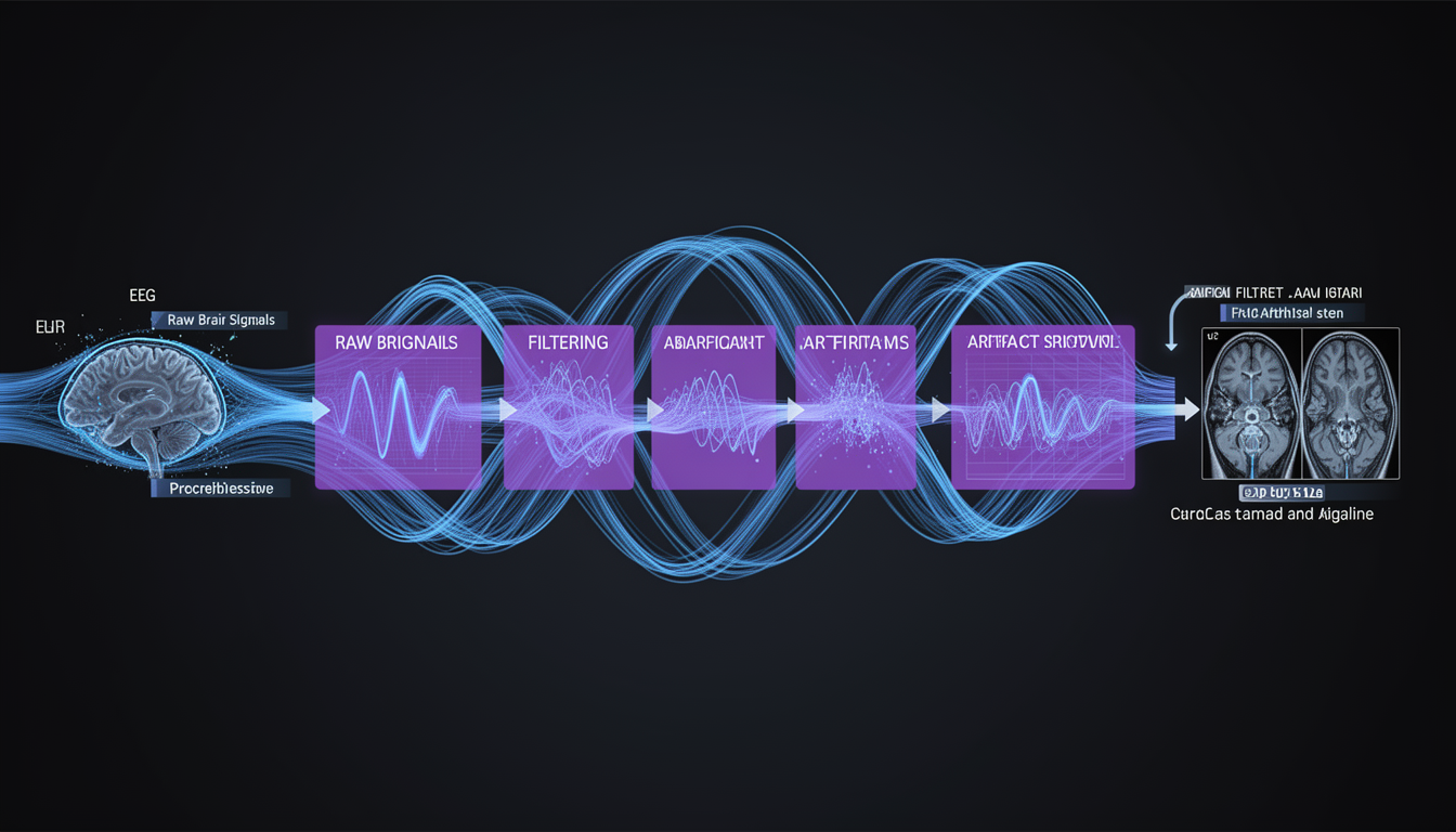
 Figure 8.1: The data science pipeline, illustrating the flow from raw neural data through preprocessing, feature extraction, and analysis to final scientific interpretation and modeling.
14.2 8.1 The Distributed Paradigm: Scaling Up Processing
Before diving into the pipeline steps, we must address a fundamental challenge: scale. Modern datasets, whether terabytes of brain imaging data or petabytes of web-scale text, are far too large for any single processor to handle. The solution, in both biology and computing, is distributed processing: breaking a massive problem into smaller pieces that can be solved in parallel.
The Brain as the Original Distributed System
The nervous system is nature’s most sophisticated distributed computing architecture. Consider what happens when you catch a ball:
Parallel sensory processing: Your visual cortex processes the ball’s trajectory, your proprioceptors track your arm’s position, and your vestibular system monitors your balance, all simultaneously.
Hierarchical delegation: Once the motor cortex plans the catch, it doesn’t micromanage every muscle fiber. Instead, it sends high-level commands to the spinal cord, which handles the low-level coordination. This is remarkably similar to how a master node dispatches tasks to worker nodes.
Reflexes as cached subroutines: When the ball touches your palm, spinal reflexes trigger grip adjustments in milliseconds, far faster than signals could travel to the brain and back. The spinal cord runs these “subroutines” locally, just as distributed systems cache frequently-used computations close to the data.
Muscle memory: When you learn to ride a bike or type on a keyboard, these motor programs become “compiled” into the cerebellum and basal ganglia, freeing your conscious mind (the “central processor”) for other tasks.
TipThe Biological Insight
The brain achieves its remarkable efficiency not by having one all-powerful processor, but by distributing specialized computations across a hierarchy of systems. The cortex handles strategy, the basal ganglia manage learned routines, and the spinal cord executes rapid reflexes. Each level operates semi-autonomously, communicating only what’s necessary.
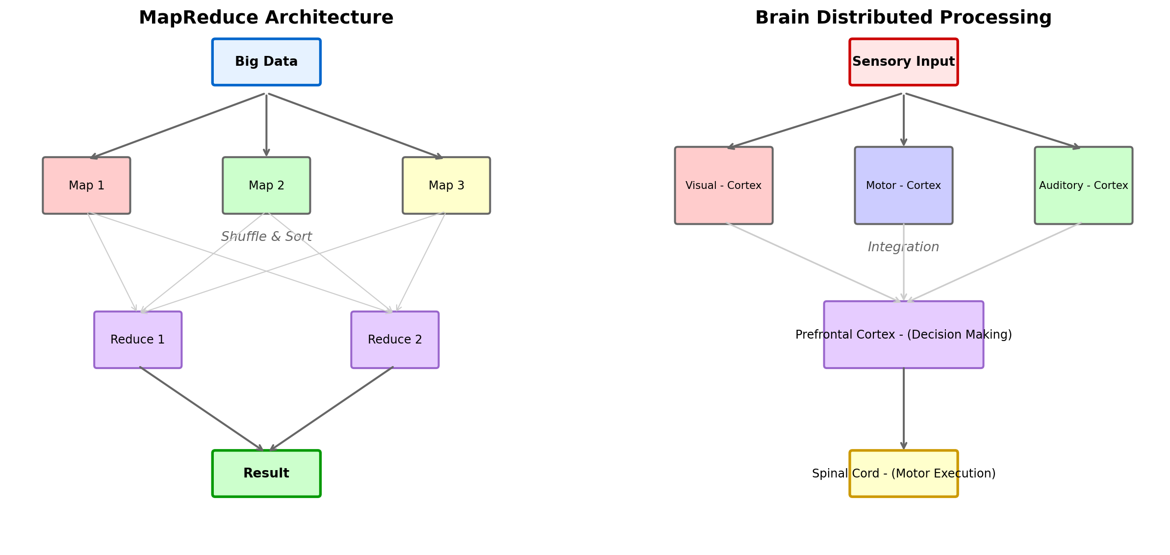
The MapReduce Paradigm: Divide and Conquer
The dominant paradigm for distributed data processing, MapReduce, mirrors this biological strategy:
Map (Divide): Split the data across many machines. Each machine processes its local chunk independently, like how different brain regions process different aspects of a scene in parallel.
Shuffle (Communicate): Intermediate results are exchanged between machines as needed, analogous to how brain regions share information through white matter tracts.
Reduce (Combine): Results are aggregated into a final answer, like how the prefrontal cortex integrates information from distributed sources to make a decision.
Figure 8.2: The parallel between MapReduce distributed computing and the brain’s hierarchical processing architecture. Both systems achieve scale by dividing work across parallel processors (map nodes / sensory cortices), exchanging only necessary information (shuffle / neural integration), and combining results at higher levels (reduce / prefrontal decision-making). The spinal cord, like edge computing, handles rapid local processing without burdening the central system.
Key Principles of Distributed Systems
Whether in silicon or neurons, distributed systems share common design principles:
| Principle | Computing Example | Neural Example |
|---|---|---|
| Data Locality | Process data where it’s stored | Reflexes handled in spinal cord |
| Fault Tolerance | Replicate data across nodes | Redundant neural pathways |
| Hierarchical Processing | Edge → Regional → Central | Spinal → Subcortical → Cortical |
| Minimal Communication | Reduce network traffic | Sparse, efficient neural coding |
| Parallel Execution | Many CPUs work simultaneously | Billions of neurons fire in parallel |
NoteWhy This Matters for Data Science
Understanding distributed processing is essential because:
- Real-world data is big: Neuroimaging datasets can reach terabytes; language models train on petabytes of text.
- The brain solves this problem daily: Evolution has optimized neural architectures for distributed processing over millions of years.
- Modern tools assume distribution: Frameworks like Spark, Dask, and PyTorch Distributed are built on these principles.
You don’t need to become a distributed systems expert, but understanding that your laptop is often not enough, and that the brain’s architecture offers design lessons, is fundamental context for modern data science.
14.3 8.2 Step 1: Acquiring and Preprocessing the Data
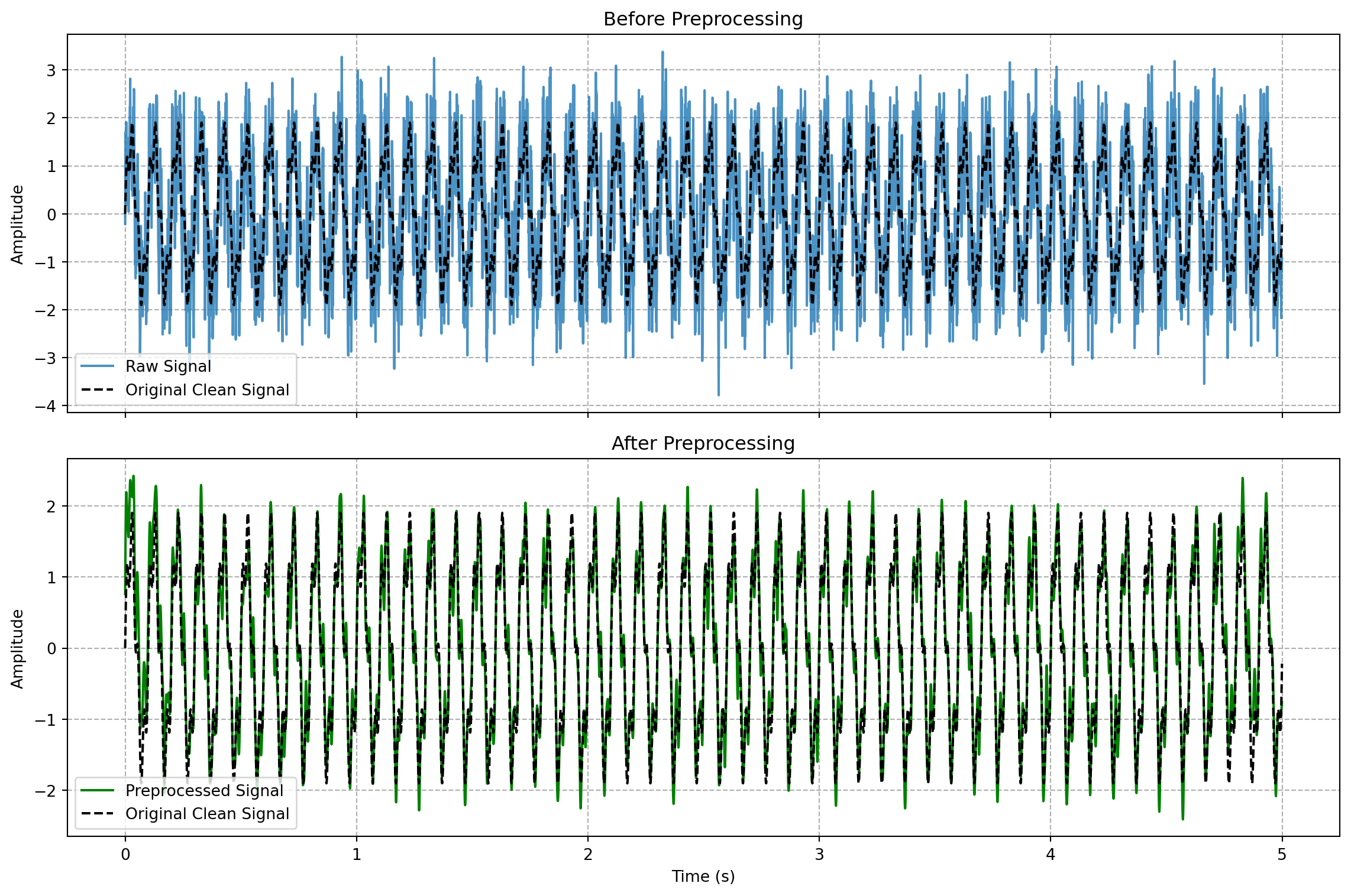
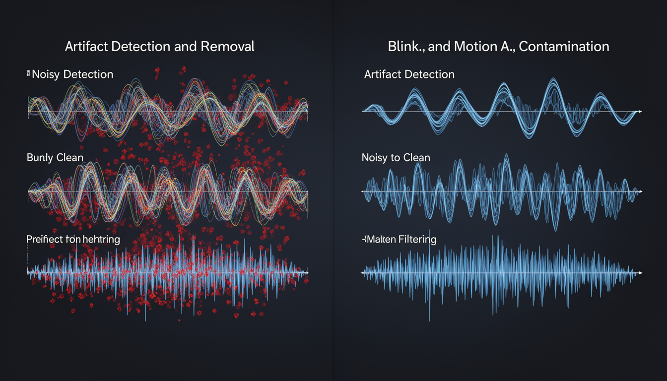
All data starts out messy. Neural recordings are contaminated by electrical noise and biological artifacts (like eye blinks or muscle movements). The first, and arguably most critical, step is to clean this data.
The Neuroscientist’s Task: Cleaning the Signal
Neural data, like Local Field Potentials (LFPs) or EEG, is often contaminated by 60 Hz electrical line noise and low-frequency drift. We use filters to remove this noise. - Band-pass filter: Keeps frequencies in a desired range (e.g., 1-100 Hz) and removes the rest. - Notch filter: Specifically removes a single frequency, like 60 Hz line noise.
The AI Engineer’s Parallel: Data Cleaning and Normalization
This is identical to the initial data cleaning phase in any machine learning project. An AI engineer might: - Remove or impute missing values. - Correct erroneous data entries. - Normalize or standardize features (e.g., using a Z-score) so that all inputs are on a similar scale. This is crucial for the stable training of deep neural networks.
Code Lab: Preprocessing a Neural Signal
Let’s simulate a raw neural signal and apply these standard preprocessing steps.
14.4 8.3 Step 2: Feature Extraction
Raw data is often not in the most informative format. Feature extraction is the art of creating new, more useful variables from the existing data.
The Neuroscientist’s Task: From Voltages to Brain Rhythms
A raw EEG signal is just a time series of voltages. A more informative feature might be the power in different frequency bands (Delta, Theta, Alpha, Beta, Gamma), as these bands are known to be associated with different cognitive states.
The AI Engineer’s Parallel: Feature Engineering
This is a classic step in machine learning. For example, when working with text data, instead of using the raw words, an engineer might extract features like: - TF-IDF scores: How important a word is to a document. - Word Embeddings (e.g., Word2Vec): A dense vector representation of a word’s meaning.
In both cases, we are transforming the data into a representation that makes the underlying patterns more apparent.
14.5 8.4 Step 3: Exploratory Analysis and Dimensionality Reduction
High-dimensional data is impossible for humans to visualize. The activity of hundreds of neurons or the feature vector of a large AI model can have thousands of dimensions. Dimensionality reduction is a set of techniques for projecting this data down into a low-dimensional space (usually 2D or 3D) that we can look at.
The Neuroscientist’s Task: Finding Neural Trajectories
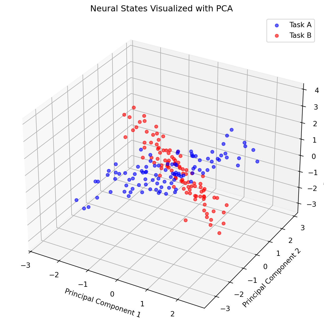
A neuroscientist might record from 100 neurons simultaneously during a task. This is a 100-dimensional space. By using a technique like Principal Component Analysis (PCA), they can find the main axes of variation in this data and plot the population activity as a “neural trajectory” through a 3D space, revealing the underlying dynamics.
The AI Engineer’s Parallel: Visualizing Embeddings
An AI engineer who has trained a language model might want to understand the relationships between the word embeddings. They can use a technique like t-SNE or UMAP to project the high-dimensional embedding vectors into a 2D plot, revealing clusters of related words.
Code Lab: Visualizing Neural States with PCA
Let’s simulate activity from a population of neurons during two different tasks and use PCA to see if we can visually separate the neural states associated with each task.
14.6 8.5 Step 4: Modeling and Decoding
The ultimate goal is often to build a model that can make predictions from the data. In neuroscience, this is called decoding: can we predict what a person is seeing, thinking, or doing based on their brain activity?
The Neuroscientist’s Task: Decoding a Subject’s Intention
A neuroscientist might train a Support Vector Machine (SVM) or a Random Forest classifier to predict whether a subject is about to press a button with their left or right hand, using EEG data from the motor cortex as input features.
The AI Engineer’s Parallel: Building a Classifier
This is the bread and butter of supervised machine learning. An AI engineer trains a model (e.g., a deep neural network) to predict a label (e.g., “cat” or “dog”) from an input (an image). The underlying process of fitting a model to a labeled dataset is identical.
14.7 8.6 Step 5: Validation and Interpretation
A model that performs well on its training data is useless if it can’t generalize to new, unseen data. Validation is the process of testing a model’s performance on a held-out dataset.
The Neuroscientist’s Task: Cross-Validation
To ensure their decoder is robust, a neuroscientist will use cross-validation. They will train their model on 80% of the data and test it on the remaining 20%, repeating this process multiple times with different splits to get a reliable estimate of its performance.
The AI Engineer’s Parallel: The Train/Validation/Test Split
This is a non-negotiable step in AI development. Data is split into a training set (for fitting the model), a validation set (for tuning hyperparameters), and a test set (for the final, unbiased evaluation of performance). The principle is exactly the same as in the neuroscience context.
14.8 8.7 Key Takeaways
- A Universal Workflow: The data science pipeline is a universal framework for turning data into knowledge, applicable to both neuroscience and AI.
- Garbage In, Garbage Out: Preprocessing and data cleaning are often the most critical steps. No amount of fancy modeling can save a project with bad data.
- Dimensionality Reduction is Key: High-dimensional data is the norm. Techniques like PCA and t-SNE are essential for visualization and building intuition.
- The Goal is Generalization: A model is only useful if it can perform well on new data. Rigorous validation is non-negotiable.
- A Shared Toolkit: Neuroscientists and AI engineers use the same core computational and statistical tools, even if they apply them to different kinds of data. Understanding this shared toolkit is a superpower.
ImportantChapter Summary
In this chapter, we walked through the five essential stages of the data science pipeline, highlighting the deep parallels between analyzing neural data and building AI systems.
- We started with Preprocessing, seeing how filtering neural signals is analogous to cleaning and normalizing data for a machine learning model.
- We moved to Feature Extraction, understanding that creating informative features—like frequency bands from an EEG signal—is a universal step in making data more useful.
- We explored Dimensionality Reduction with PCA, visualizing how we can find meaningful structure in high-dimensional neural data, just as an AI engineer visualizes word embeddings.
- We discussed Modeling and Decoding, framing the process of predicting a stimulus from brain activity as a standard supervised learning problem.
- Finally, we emphasized the critical importance of Validation, showing how techniques like cross-validation ensure that our models are robust and can generalize to new data.
By understanding this shared pipeline, you are now equipped with a mental model that can guide you through any data-driven project, from analyzing a single neuron to training a large language model.
14.9 8.8 Exercises
Conceptual Questions
Describe the five stages of the data science pipeline. For each stage (acquisition & preprocessing, feature extraction, exploratory analysis, modeling, and validation), explain its purpose and why it’s essential. What can go wrong if any stage is skipped or done poorly?
Compare signal preprocessing in neuroscience vs. data cleaning in AI. What are the parallels between filtering neural signals and normalizing features for machine learning? Why is the principle “garbage in, garbage out” universal across both domains?
Explain the purpose of dimensionality reduction. Why is it necessary for both visualization and computation? Compare PCA (linear) and t-SNE (nonlinear) - when would you use each?
Discuss the importance of proper validation. What is the difference between training, validation, and test sets? Why is cross-validation better than a single train-test split? What happens if you “peek” at the test set during model development?
Computational Problems
- Build a complete preprocessing pipeline for neural data. Using simulated EEG or LFP data:
- Remove 60 Hz line noise with a notch filter
- Apply a bandpass filter (1-100 Hz)
- Detect and remove artifacts (e.g., values exceeding 5 standard deviations)
- Normalize the signal (z-score)
- Visualize each preprocessing step and quantify its effect
- Extract and compare features from neural signals. Given a multi-channel neural recording:
- Extract time-domain features (mean, variance, peak amplitude)
- Extract frequency-domain features (power in different bands: delta, theta, alpha, beta, gamma)
- Use PCA to identify which features carry the most variance
- Build a simple classifier using different feature sets and compare performance
- Implement dimensionality reduction on population activity. Simulate:
- Activity from 100 neurons during two different behavioral states
- Apply PCA to reduce to 3 dimensions
- Apply t-SNE and UMAP for comparison
- Visualize the neural trajectories in reduced space
- Quantify how much variance is preserved by each method
- Build and validate a neural decoder. Create:
- A simulated dataset of neural activity paired with stimulus labels
- Train multiple classifiers (logistic regression, SVM, random forest)
- Implement k-fold cross-validation
- Plot learning curves (performance vs. training set size)
- Analyze which neural features the best model relies on most
Discussion Questions
- Transfer learning: From computer vision to neuroscience. The data science pipeline is similar across domains. Discuss:
- How could techniques from computer vision (e.g., data augmentation, transfer learning) be applied to neural data analysis?
- What are the challenges in transferring methods between domains?
- Could pre-trained models on large neural datasets accelerate future neuroscience research?
- What would a “ImageNet for neuroscience” look like?
- Interpretability vs. performance trade-offs. In both neuroscience and AI:
- Why might a simple linear model be preferable to a complex deep network, even if it’s less accurate?
- How do we balance model interpretability with predictive power?
- What techniques can make complex models more interpretable (e.g., feature importance, attention visualization)?
- When is interpretability crucial, and when is pure prediction sufficient?
- Reproducibility in data science. Both neuroscience and AI face reproducibility challenges. Discuss:
- What practices ensure reproducible data analysis (version control, random seeds, containerization)?
- How can we share both code and data in ways that enable others to verify and build on our work?
- What are the ethical implications of irreproducible research?
- How might standards for reproducibility differ between academic neuroscience and industry AI?
14.10 8.9 References
Dean, J., & Ghemawat, S. (2008). MapReduce: Simplified data processing on large clusters. Communications of the ACM, 51(1), 107-113.
Bullmore, E., & Sporns, O. (2012). The economy of brain network organization. Nature Reviews Neuroscience, 13(5), 336-349.
McKinney, W. (2017). Python for Data Analysis: Data Wrangling with Pandas, NumPy, and IPython (2nd ed.). O’Reilly Media.
Géron, A. (2019). Hands-On Machine Learning with Scikit-Learn, Keras, and TensorFlow (2nd ed.). O’Reilly Media.
Cohen, M. X. (2014). Analyzing Neural Time Series Data: Theory and Practice. MIT Press.
Kramer, M. A., & Eden, U. T. (2016). Case Studies in Neural Data Analysis: A Guide for the Practicing Neuroscientist. MIT Press.
Gramfort, A., Luessi, M., Larson, E., Engemann, D. A., Strohmeier, D., Brodbeck, C., et al. (2013). MEG and EEG data analysis with MNE-Python. Frontiers in Neuroscience, 7, 267.
Pedregosa, F., Varoquaux, G., Gramfort, A., Michel, V., Thirion, B., Grisel, O., et al. (2011). Scikit-learn: Machine learning in Python. Journal of Machine Learning Research, 12, 2825-2830.
VanderPlas, J. (2016). Python Data Science Handbook: Essential Tools for Working with Data. O’Reilly Media.
Hastie, T., Tibshirani, R., & Friedman, J. (2009). The Elements of Statistical Learning: Data Mining, Inference, and Prediction (2nd ed.). Springer.
Cunningham, J. P., & Byron, M. Y. (2014). Dimensionality reduction for large-scale neural recordings. Nature Neuroscience, 17(11), 1500-1509.
Paninski, L., & Cunningham, J. P. (2018). Neural data science: Accelerating the experiment-analysis-theory cycle in large-scale neuroscience. Current Opinion in Neurobiology, 50, 232-241.
Glaser, J. I., Benjamin, A. S., Farhoodi, R., & Kording, K. P. (2019). The roles of supervised machine learning in systems neuroscience. Progress in Neurobiology, 175, 126-137.
Stevenson, I. H., & Kording, K. P. (2011). How advances in neural recording affect data analysis. Nature Neuroscience, 14(2), 139-142.