import numpy as np
import matplotlib.pyplot as plt
from scipy.stats import beta

def bayesian_coin_flip(n_flips=20, true_prob=0.7, show_animation=False):
    """
    Demonstrate Bayesian inference for estimating the bias of a coin.

    Prior: Beta(2, 2) - slightly peaked at 0.5
    Likelihood: Binomial(n_flips, θ)
    Posterior: Beta(α + n_heads, β + n_tails)

    This is conjugate: Beta prior + Binomial likelihood = Beta posterior
    """
    np.random.seed(42)

    # Generate coin flips
    flips = np.random.rand(n_flips) < true_prob  # True if heads
    n_heads = np.cumsum(flips)
    n_tails = np.arange(1, n_flips+1) - n_heads

    # Prior parameters (Beta distribution)
    alpha_prior = 2
    beta_prior = 2

    # Create θ values for plotting
    theta = np.linspace(0, 1, 1000)

    # Plot evolution of belief
    fig, axes = plt.subplots(2, 2, figsize=(14, 10))
    axes = axes.ravel()

    plot_points = [0, 4, 9, n_flips-1]  # Which flips to show

    for idx, flip_idx in enumerate(plot_points):
        ax = axes[idx]

        if flip_idx == 0:
            # Prior only
            alpha_post = alpha_prior
            beta_post = beta_prior
            n_h = 0
            n_t = 0
        else:
            # Posterior after flip_idx flips
            alpha_post = alpha_prior + n_heads[flip_idx]
            beta_post = beta_prior + n_tails[flip_idx]
            n_h = n_heads[flip_idx]
            n_t = n_tails[flip_idx]

        # Plot posterior
        post_dist = beta.pdf(theta, alpha_post, beta_post)
        ax.plot(theta, post_dist, 'b-', linewidth=2, label='Posterior')
        ax.fill_between(theta, post_dist, alpha=0.3, color='blue')

        # True value
        ax.axvline(true_prob, color='red', linestyle='--',
                   linewidth=2, label=f'True θ = {true_prob}')

        # MAP estimate
        map_estimate = (alpha_post - 1) / (alpha_post + beta_post - 2)
        ax.axvline(map_estimate, color='green', linestyle='-',
                   linewidth=2, label=f'MAP = {map_estimate:.2f}')

        ax.set_xlabel('θ (Probability of Heads)')
        ax.set_ylabel('Probability Density')
        ax.set_title(f'After {n_h} heads, {n_t} tails')
        ax.legend()
        ax.grid(alpha=0.3)
        ax.set_ylim(0, ax.get_ylim()[1] * 1.1)

    plt.tight_layout()

    print(f"True probability: {true_prob}")
    print(f"Final MAP estimate: {map_estimate:.3f}")
    print(f"Final posterior: Beta({alpha_post}, {beta_post})")

    return alpha_post, beta_post

# bayesian_coin_flip(n_flips=20, true_prob=0.7)17 Bayesian Decision Making
NoteLearning Objectives
By the end of this chapter, you will be able to:
- Understand the Bayesian brain hypothesis and its implications
- Apply Bayes’ rule to update beliefs in light of new evidence
- Implement Bayesian inference algorithms for perception and decision-making
- Compute optimal decisions using expected utility theory
- Connect Bayesian models to neural computation and behavior
- Evaluate Bayesian models of sensory integration and multisensory perception
17.1 11.1 The Bayesian Brain Hypothesis
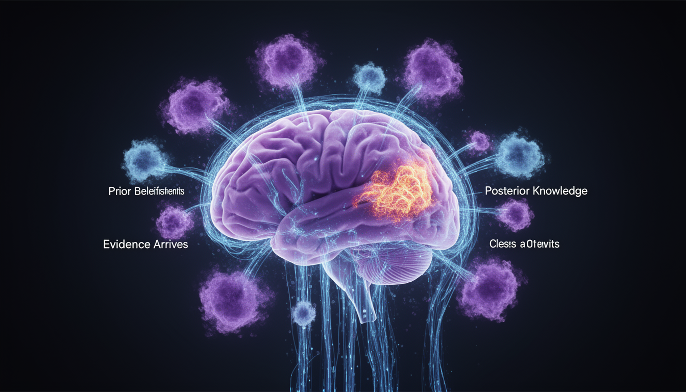
How do we make decisions in a world that is fundamentally uncertain? The Bayesian brain hypothesis proposes that the brain represents knowledge about the world in the form of probability distributions and that it uses the principles of Bayesian inference to update these beliefs in the light of new evidence.
This is a powerful idea because it provides a normative framework for understanding how an ideal observer should reason and make decisions under uncertainty. By comparing the behavior of humans and animals to the predictions of Bayesian models, we can gain insights into the computational principles that underlie perception, cognition, and action. While Chapter 9 focused on causal inference (determining what causes what), this chapter focuses on probabilistic inference (updating beliefs under uncertainty) - two complementary approaches to reasoning about the world.
Why Bayesian? The Problem of Uncertainty
The world is inherently noisy and ambiguous: - Sensory signals are corrupted by neural noise - The same sensation can arise from different causes - We have incomplete information about the world
Example: Imagine you see a shadowy figure in the dark. Is it a person, a tree, or just a trick of the light? Your brain must integrate: - Current sensory evidence (what you see now) - Prior knowledge (how common are trees vs. intruders?) - Context (are you in a forest or a parking lot?)
Bayesian inference provides the optimal solution to this problem.
17.2 11.2 The Core of Bayesian Inference
At the heart of Bayesian inference is Bayes’ rule, which describes how to update our beliefs about a hypothesis in the light of new data. The rule is surprisingly simple:
\[ P(H|D) = \frac{P(D|H)P(H)}{P(D)} \]
Let’s break down the terms:
- \(P(H)\) (The Prior): This is our initial belief about the hypothesis before we see any data. It represents our prior knowledge about the world.
- \(P(D|H)\) (The Likelihood): This is the probability of observing the data given that the hypothesis is true. It’s a model of how the data is generated.
- \(P(D)\) (The Evidence): This is the total probability of observing the data, averaged over all possible hypotheses. It acts as a normalization constant.
- \(P(H|D)\) (The Posterior): This is our updated belief about the hypothesis after we have seen the data. It’s the result of combining our prior with the likelihood.
In essence, Bayes’ rule tells us how to combine what we already know (the prior) with what we’ve just learned (the likelihood) to form a new, more informed belief (the posterior).
 Figure 11.1: Bayes’ Rule for updating beliefs. The posterior combines prior knowledge P(H) with new evidence via the likelihood P(D|H), normalized by P(D). This is the foundation of Bayesian inference.

Code Lab: Bayesian Coin Flip
Key Insight: As we gather more evidence (flips), the posterior becomes more concentrated around the true value.
 Figure 11.3: Sequential Bayesian belief updating. Starting from a broad prior (no data), the posterior distribution narrows and converges toward the true value as evidence accumulates. The MAP estimate improves with each observation, demonstrating how Bayesian inference learns from experience. The prior matters most when data is scarce, but eventually the data overwhelms the prior.
The Conjugate Prior Trick
In the coin flip example, we used a conjugate prior: a Beta prior with a Binomial likelihood yields a Beta posterior. This makes the math tractable and allows us to update our beliefs efficiently.
Common conjugate pairs: - Beta-Binomial (coin flips, binary choices) - Gamma-Poisson (neural spike counts) - Normal-Normal (continuous measurements)
17.3 11.3 Bayesian Perception: Combining Sensory Cues
One of the most compelling applications of Bayesian inference in neuroscience is sensory cue integration. How does the brain combine information from multiple senses?
The Optimal Cue Integration Model
When combining two noisy estimates \(x_1\) and \(x_2\) with variances \(\sigma_1^2\) and \(\sigma_2^2\), the optimal Bayesian estimate is:
\[ \hat{x} = w_1 x_1 + w_2 x_2 \]
where the weights are proportional to the inverse variances (precision):
\[ w_1 = \frac{\sigma_2^2}{\sigma_1^2 + \sigma_2^2}, \quad w_2 = \frac{\sigma_1^2}{\sigma_1^2 + \sigma_2^2} \]
Key principle: More reliable (less noisy) cues get higher weight.
 Figure 11.2: Optimal Bayesian sensory cue integration. Visual and haptic estimates are combined with weights proportional to their reliabilities (inverse variances). The combined estimate is more precise than either modality alone, a prediction confirmed by human psychophysics experiments.
def multisensory_integration():
    """
    Demonstrate optimal Bayesian cue integration.

    Scenario: Estimate object size using vision and touch.
    - Visual estimate: noisy but available
    - Haptic (touch) estimate: also noisy
    - Optimal strategy: weight by reliability (inverse variance)
    """
    np.random.seed(42)

    # True object size
    true_size = 10.0  # cm

    # Generate repeated measurements
    n_trials = 100

    # Visual measurements (more variable)
    visual_noise_std = 2.0
    visual_estimates = true_size + np.random.randn(n_trials) * visual_noise_std

    # Haptic measurements (less variable)
    haptic_noise_std = 1.0
    haptic_estimates = true_size + np.random.randn(n_trials) * haptic_noise_std

    # Optimal Bayesian combination
    visual_precision = 1 / visual_noise_std**2
    haptic_precision = 1 / haptic_noise_std**2

    w_visual = visual_precision / (visual_precision + haptic_precision)
    w_haptic = haptic_precision / (visual_precision + haptic_precision)

    combined_estimates = w_visual * visual_estimates + w_haptic * haptic_estimates

    # Sub-optimal: equal weighting
    equal_weight_estimates = 0.5 * visual_estimates + 0.5 * haptic_estimates

    # Visualization
    fig, axes = plt.subplots(1, 2, figsize=(14, 6))

    # Plot 1: Individual and combined estimates
    axes[0].scatter(visual_estimates, haptic_estimates, alpha=0.3, c='gray')
    axes[0].scatter(combined_estimates.mean(), combined_estimates.mean(),
                   s=200, c='green', marker='*', label='Bayesian combined',
                   edgecolors='black', linewidths=2)
    axes[0].scatter(true_size, true_size, s=200, c='red', marker='X',
                   label='True value', edgecolors='black', linewidths=2)
    axes[0].set_xlabel('Visual Estimate (cm)')
    axes[0].set_ylabel('Haptic Estimate (cm)')
    axes[0].set_title('Multisensory Integration')
    axes[0].legend()
    axes[0].grid(alpha=0.3)
    axes[0].axis('equal')

    # Plot 2: Error distributions
    visual_errors = np.abs(visual_estimates - true_size)
    haptic_errors = np.abs(haptic_estimates - true_size)
    combined_errors = np.abs(combined_estimates - true_size)
    equal_errors = np.abs(equal_weight_estimates - true_size)

    positions = [1, 2, 3, 4]
    data = [visual_errors, haptic_errors, combined_errors, equal_errors]
    labels = ['Visual - only', 'Haptic - only', 'Bayesian - combined', 'Equal - weight']

    bp = axes[1].boxplot(data, positions=positions, labels=labels,
                         patch_artist=True, widths=0.6)

    colors = ['#cc0000', '#0066cc', '#00cc00', '#cccccc']
    for patch, color in zip(bp['boxes'], colors):
        patch.set_facecolor(color)
        patch.set_alpha(0.7)

    axes[1].set_ylabel('Absolute Error (cm)')
    axes[1].set_title('Estimation Error by Strategy')
    axes[1].grid(alpha=0.3, axis='y')

    plt.tight_layout()

    print(f"Visual weight: {w_visual:.3f}")
    print(f"Haptic weight: {w_haptic:.3f}")
    print(f" - Mean absolute errors:")
    print(f"  Visual only: {visual_errors.mean():.3f} cm")
    print(f"  Haptic only: {haptic_errors.mean():.3f} cm")
    print(f"  Bayesian combined: {combined_errors.mean():.3f} cm")
    print(f"  Equal weight: {equal_errors.mean():.3f} cm")

    return w_visual, w_haptic

# multisensory_integration()
Neuroscience Evidence: Ernst & Banks (2002) showed that humans optimally combine visual and haptic cues for size estimation, with weights matching the Bayesian prediction.
17.4 11.4 Making Decisions with Utility
Once we have a posterior distribution that represents our beliefs about the state of the world, how do we use it to make a decision? This is where the concept of utility comes in.
A utility function, \(U(s, a)\), quantifies the value of taking a particular action, \(a\), when the true state of the world is \(s\). To make an optimal decision, we should choose the action that maximizes our expected utility, which is the average of the utility function weighted by the posterior probability of each state:
\[ \mathbb{E}[U(a)] = \sum_s U(s, a) P(s|D) \]
By combining Bayesian inference with the principle of maximum expected utility, we have a complete framework for making optimal decisions under uncertainty.
 Figure 11.4: Bayesian decision making maximizes expected utility. For each action, we compute the expected utility by weighing outcomes by their posterior probabilities. The optimal decision (Wait: E[U]=7.0 > Treat: E[U]=6.6) accounts for both uncertainty about the world state and the utilities of different outcomes.
Code Lab: Perceptual Decision Making
def perceptual_decision_making():
    """
    Simulate Bayesian perceptual decision making.

    Task: Decide whether a noisy stimulus is 'A' or 'B'
    - Collect evidence over time
    - Update posterior probability
    - Make decision when confidence threshold is reached
    """
    np.random.seed(42)

    # True stimulus (0 = A, 1 = B)
    true_stimulus = 1

    # Evidence parameters
    n_timesteps = 50
    if true_stimulus == 0:
        evidence_mean = -0.3  # Evidence favors A
    else:
        evidence_mean = +0.3  # Evidence favors B
    evidence_std = 1.0

    # Prior (equal probability)
    prior_A = 0.5
    prior_B = 0.5

    # Collect evidence over time
    evidence = evidence_mean + np.random.randn(n_timesteps) * evidence_std
    cumulative_evidence = np.cumsum(evidence)

    # Update posterior using Bayesian inference
    # For simplicity, using a diffusion model approximation
    posterior_B = np.zeros(n_timesteps)
    log_posterior_ratio = np.zeros(n_timesteps)

    for t in range(n_timesteps):
        # Log likelihood ratio
        log_lr = cumulative_evidence[t] / evidence_std**2

        # Log posterior ratio (log odds)
        log_posterior_ratio[t] = log_lr + np.log(prior_B / prior_A)

        # Convert to probability
        posterior_B[t] = 1 / (1 + np.exp(-log_posterior_ratio[t]))

    # Decision rule: choose when posterior exceeds threshold
    confidence_threshold = 0.95
    decision_time = np.where(posterior_B > confidence_threshold)[0]

    if len(decision_time) > 0:
        decision_time = decision_time[0]
        decision = 'B'
    elif len(np.where(posterior_B < 1 - confidence_threshold)[0]) > 0:
        decision_time = np.where(posterior_B < 1 - confidence_threshold)[0][0]
        decision = 'A'
    else:
        decision_time = n_timesteps - 1
        decision = 'B' if posterior_B[-1] > 0.5 else 'A'

    # Visualization
    fig, axes = plt.subplots(2, 1, figsize=(12, 10))

    # Plot 1: Evidence accumulation
    axes[0].plot(cumulative_evidence, 'b-', linewidth=2, label='Cumulative evidence')
    axes[0].axhline(0, color='gray', linestyle='--', alpha=0.5)
    axes[0].axvline(decision_time, color='red', linestyle='--',
                    label=f'Decision time = {decision_time}')
    axes[0].set_xlabel('Time (ms)')
    axes[0].set_ylabel('Cumulative Evidence')
    axes[0].set_title('Evidence Accumulation Over Time')
    axes[0].legend()
    axes[0].grid(alpha=0.3)

    # Plot 2: Posterior probability
    axes[1].plot(posterior_B, 'g-', linewidth=2, label='P(stimulus = B | evidence)')
    axes[1].axhline(0.5, color='gray', linestyle='--', alpha=0.5, label='Chance')
    axes[1].axhline(confidence_threshold, color='red', linestyle=':',
                    alpha=0.7, label=f'Threshold = {confidence_threshold}')
    axes[1].axhline(1 - confidence_threshold, color='red', linestyle=':', alpha=0.7)
    axes[1].axvline(decision_time, color='red', linestyle='--')
    axes[1].set_xlabel('Time (ms)')
    axes[1].set_ylabel('Posterior Probability')
    axes[1].set_title('Bayesian Belief Update')
    axes[1].set_ylim(0, 1)
    axes[1].legend()
    axes[1].grid(alpha=0.3)

    plt.tight_layout()

    correct = (decision == 'B' and true_stimulus == 1) or (decision == 'A' and true_stimulus == 0)
    print(f"True stimulus: {'B' if true_stimulus == 1 else 'A'}")
    print(f"Decision: {decision}")
    print(f"Decision time: {decision_time} ms")
    print(f"Correct: {correct}")

    return decision, decision_time

# perceptual_decision_making()
Connection to Neuroscience: This model resembles the drift-diffusion model, which accurately describes reaction times and choice behavior in perceptual decision-making tasks. Neural recordings in areas like LIP and FEF show evidence accumulation patterns matching this model.
17.5 11.5 Bayesian Brain: Neural Implementation
How might neurons implement Bayesian inference? Several theories have been proposed:
Probabilistic Population Codes
One idea is that populations of neurons encode probability distributions: - Mean: Encoded in the population average - Variance/uncertainty: Encoded in the population variance or correlation structure
def probabilistic_population_code():
    """
    Demonstrate how a neural population can encode a probability distribution.

    Population coding: Each neuron has a preferred stimulus value (tuning curve)
    Population activity pattern represents posterior distribution
    """
    np.random.seed(42)

    # Stimulus space
    stimulus_values = np.linspace(0, 180, 100)  # Orientation in degrees

    # Neural population
    n_neurons = 20
    preferred_orientations = np.linspace(0, 180, n_neurons)
    tuning_width = 20  # degrees

    # True stimulus
    true_orientation = 90

    # Noisy sensory input
    noisy_measurement = true_orientation + np.random.randn() * 10

    # Generate population response
    def tuning_curve(stimulus, preferred, width):
        """Gaussian tuning curve."""
        return np.exp(-0.5 * ((stimulus - preferred) / width)**2)

    population_response = np.zeros(n_neurons)
    for i in range(n_neurons):
        mean_response = tuning_curve(noisy_measurement,
                                     preferred_orientations[i],
                                     tuning_width)
        # Add Poisson noise
        population_response[i] = np.random.poisson(mean_response * 100)

    # Decode: Reconstruct probability distribution from population
    likelihood = np.zeros(len(stimulus_values))
    for i in range(n_neurons):
        # Each neuron votes for stimuli near its preferred orientation
        contribution = tuning_curve(stimulus_values,
                                   preferred_orientations[i],
                                   tuning_width)
        likelihood += contribution * population_response[i]

    # Normalize to get posterior (assuming flat prior)
    posterior = likelihood / likelihood.sum()

    # Maximum a posteriori (MAP) estimate
    map_estimate = stimulus_values[np.argmax(posterior)]

    # Visualization
    fig, axes = plt.subplots(2, 1, figsize=(12, 10))

    # Plot 1: Population response
    axes[0].bar(preferred_orientations, population_response,
               width=8, color='#cc0000', alpha=0.7)
    axes[0].axvline(true_orientation, color='green', linestyle='--',
                   linewidth=2, label=f'True orientation = {true_orientation}°')
    axes[0].set_xlabel('Preferred Orientation (degrees)')
    axes[0].set_ylabel('Spike Count')
    axes[0].set_title('Neural Population Response')
    axes[0].legend()
    axes[0].grid(alpha=0.3, axis='y')

    # Plot 2: Decoded posterior
    axes[1].plot(stimulus_values, posterior, 'b-', linewidth=2,
                label='Decoded posterior')
    axes[1].fill_between(stimulus_values, posterior, alpha=0.3, color='blue')
    axes[1].axvline(true_orientation, color='green', linestyle='--',
                   linewidth=2, label=f'True = {true_orientation}°')
    axes[1].axvline(map_estimate, color='red', linestyle='-',
                   linewidth=2, label=f'MAP = {map_estimate:.1f}°')
    axes[1].set_xlabel('Orientation (degrees)')
    axes[1].set_ylabel('Probability Density')
    axes[1].set_title('Decoded Posterior Distribution')
    axes[1].legend()
    axes[1].grid(alpha=0.3)

    plt.tight_layout()

    print(f"True orientation: {true_orientation}°")
    print(f"Noisy measurement: {noisy_measurement:.1f}°")
    print(f"MAP estimate: {map_estimate:.1f}°")
    print(f"Estimation error: {abs(map_estimate - true_orientation):.1f}°")

    return population_response, posterior

# probabilistic_population_code()
Predictive Coding
Another influential theory is predictive coding: the brain constantly generates predictions about sensory inputs and only propagates prediction errors up the hierarchy.
Key idea: - Top-down: Predictions (prior expectations) - Bottom-up: Prediction errors (deviations from expectations) - Learning: Update internal models to minimize prediction errors
This framework elegantly combines Bayesian inference with hierarchical processing.
17.6 11.6 Challenges and Limitations
While the Bayesian brain hypothesis is powerful, it faces several challenges:
Computational Intractability: Exact Bayesian inference is computationally expensive for complex problems. The brain must use approximations.
Where do priors come from? Are they innate, learned, or both?
Neural implementation: The exact neural mechanisms for probabilistic computation remain unclear.
Deviations from optimality: Humans often deviate from Bayesian predictions (e.g., base rate neglect, confirmation bias).
These challenges don’t invalidate the framework but highlight that the brain may implement approximate Bayesian inference rather than exact computation.
17.7 Exercises
Conceptual Questions
Bayes vs. Frequentist: Explain the key difference between Bayesian and frequentist approaches to statistics. Why might the brain be “Bayesian”?
Prior Knowledge: In Bayesian inference, where do priors come from? Give examples of priors that might be innate vs. learned through experience.
Cue Integration: Why is it optimal to weight sensory cues by their reliability (inverse variance)? What would happen if the brain used equal weights?
Computational Problems
Medical Diagnosis: A disease affects 1% of the population. A test is 95% sensitive (true positive rate) and 90% specific (true negative rate). If you test positive, what’s the probability you have the disease? Solve using Bayes’ rule.
Bayesian Updating: Implement a Bayesian model that estimates the mean of a Gaussian distribution from noisy samples. Start with a prior, then update it sequentially as new data arrives. Plot the evolution of the posterior.
Optimal Cue Integration: Generate synthetic data for two sensory modalities with different noise levels. Implement optimal Bayesian cue integration and compare its performance to using each modality alone or equal weighting.
Sequential Decision Making: Implement a drift-diffusion model for a two-alternative forced choice task. Vary the evidence strength and decision threshold, and plot reaction time distributions.
Discussion Questions
Neural Implementation: How might neurons implement Bayesian inference? Discuss different proposals (population codes, sampling, neural networks).
Approximate Inference: Exact Bayesian inference is often intractable. What approximations might the brain use? (Hint: particle filters, variational inference, sampling)
Bias and Rationality: Humans often deviate from Bayesian optimality (e.g., overconfidence, base rate neglect). Are these true irrationalities, or could they be rational under resource constraints?
17.8 References
Doya, K., Ishii, S., Pouget, A., & Rao, R. P. N. (Eds.). (2007). Bayesian Brain: Probabilistic Approaches to Neural Coding. MIT Press.
Knill, D. C., & Pouget, A. (2004). The Bayesian brain: The role of uncertainty in neural coding and computation. Trends in Neurosciences, 27(12), 712-719.
Ma, W. J., Beck, J. M., Latham, P. E., & Pouget, A. (2006). Bayesian inference with probabilistic population codes. Nature Neuroscience, 9(11), 1432-1438.
Ernst, M. O., & Banks, M. S. (2002). Humans integrate visual and haptic information in a statistically optimal fashion. Nature, 415(6870), 429-433.
Körding, K. P., & Wolpert, D. M. (2004). Bayesian integration in sensorimotor learning. Nature, 427(6971), 244-247.
Rao, R. P., & Ballard, D. H. (1999). Predictive coding in the visual cortex: A functional interpretation of some extra-classical receptive-field effects. Nature Neuroscience, 2(1), 79-87.
Friston, K. (2010). The free-energy principle: A unified brain theory? Nature Reviews Neuroscience, 11(2), 127-138.
Gold, J. I., & Shadlen, M. N. (2007). The neural basis of decision making. Annual Review of Neuroscience, 30, 535-574.
Tenenbaum, J. B., Kemp, C., Griffiths, T. L., & Goodman, N. D. (2011). How to grow a mind: Statistics, structure, and abstraction. Science, 331(6022), 1279-1285.
Gershman, S. J., Horvitz, E. J., & Tenenbaum, J. B. (2015). Computational rationality: A converging paradigm for intelligence in brains, minds, and machines. Science, 349(6245), 273-278.