35  Embodied AI: Intelligence Needs a Body

Learning Objectives By the end of this chapter, you will be able to:

• Understand the “Embodiment Hypothesis” and why physical interaction is critical for intelligence.
• Explain how the brain learns to control a complex body using principles like motor primitives and forward models.
• Analyze real-world robotics systems (Boston Dynamics, soft robotics, sim-to-real) and their neuroscience inspiration.
• Implement robotic control algorithms including inverse kinematics, trajectory planning, and active inference.
• Describe how developmental robotics replicates infant learning through curiosity-driven exploration.
• Connect predictive processing theory to motor control and optimal feedback control.
• Appreciate how perception is fundamentally action-oriented through the concept of affordances.
• Evaluate the challenges and neuroscience-inspired solutions for human-robot collaboration.

35.1 25.1 The Embodiment Hypothesis

Figure 35.1: The sensorimotor loop - the continuous cycle of perception, prediction, and action that underlies embodied intelligence.

Why a Brain in a Vat Is Not Enough

Figure 35.2: Embodied AI systems learn through sensorimotor interaction with the physical world.

For the last decade, the dominant paradigm in AI has been disembodied. Large language models are like brilliant “brains in vats,” trained on vast, static snapshots of the internet. They have never touched an object, moved through a room, or felt the consequences of an action. Biological intelligence, in contrast, is fundamentally embodied. Every thought, concept, and skill we have is shaped by the constant, dynamic interaction between our brain, our body, and the physical world.

The Embodiment Hypothesis posits that this is not a coincidence. It argues that true, general-purpose intelligence requires a body. Cognition is not just about abstract symbol manipulation; it is grounded in the rich, messy, real-time feedback loop of sensing and acting in the world.

This chapter explores the field of embodied AI and robotics, which seeks to build intelligent systems that learn, perceive, and act as physical agents in the world, drawing deep inspiration from the way the brain controls the body.

35.2 25.2 The Body as a Teacher: Sensorimotor Learning

The most fundamental source of knowledge about the world is the sensorimotor loop: the closed loop of act -> sense -> learn -> repeat. An infant learns about gravity not by reading a textbook, but by dropping a toy and observing the consequence. This physical interaction provides an endless stream of self-supervised data that grounds learning in physical reality.

Figure 35.3: Multimodal sensory integration in embodied AI - visual, auditory, and tactile information converging into unified perception.

25.2.1 The Core Loop

An embodied agent is defined by its ability to perform this loop: 1. Sense: Gather information about the state of the world and its own body through sensors (vision, touch, proprioception). 2. Act: Execute an action that changes the state of the world or its body using actuators (motors, grippers). 3. Learn: Update its internal model of the world based on the relationship between its action and the resulting sensory change.

This loop is the engine of all biological learning, and it is the foundation of modern reinforcement learning and robotics.

35.3 25.3 Case Study 1: Boston Dynamics - From Brain to Biped

Boston Dynamics’ Atlas robot represents one of the most striking examples of biological principles translated into engineered systems. Standing 1.5 meters tall and weighing 89 kg, Atlas can run, jump, do backflips, and navigate complex terrain with a fluidity that was considered impossible just a decade ago. The secret lies not just in advanced hardware, but in control algorithms inspired by the neural circuits that govern animal locomotion.

25.3.1 Central Pattern Generators for Locomotion

One of Atlas’s key innovations is the use of Central Pattern Generators (CPGs), neural circuits originally discovered in the spinal cords of animals. CPGs are rhythmic neural networks that can produce coordinated, oscillatory motor patterns without requiring continuous input from higher brain centers. In lamprey, for example, a chain of CPG circuits in the spinal cord generates the undulating swimming motion, even when the spinal cord is isolated from the brain.

Atlas uses computational CPGs—coupled oscillators that generate rhythmic leg movements for walking, running, and jumping. These CPGs provide several advantages:

• Stability: The oscillatory nature of CPGs naturally produces smooth, periodic gaits. Unlike frame-by-frame trajectory optimization, CPGs generate continuous, stable movement patterns.
• Adaptability: By modulating the frequency and amplitude of the oscillators, Atlas can seamlessly transition between walking and running, or adjust its gait for different terrains.
• Efficiency: CPGs reduce the dimensionality of the control problem. Instead of controlling dozens of joint angles independently, the controller modulates a handful of CPG parameters.

The mathematical model of a CPG can be represented as a system of coupled oscillators:

\[ \ddot{\theta}_i + 2\zeta\omega_i\dot{\theta}_i + \omega_i^2\theta_i = \sum_{j} w_{ij}\sin(\theta_j - \theta_i - \phi_{ij}) + F_{ext} \]

where \(\theta_i\) is the phase of oscillator \(i\), \(\omega_i\) is its natural frequency, \(\zeta\) is damping, \(w_{ij}\) represents coupling strength between oscillators, and \(\phi_{ij}\) is the desired phase offset. The external force \(F_{ext}\) allows sensory feedback to modulate the pattern.

25.3.2 Adaptive Balance and Terrain Negotiation

Balance control in Atlas draws inspiration from the vestibular system and cerebellar control loops in the human brain. The robot continuously integrates information from:

• IMU (Inertial Measurement Unit): Analogous to the vestibular system, providing information about orientation and angular velocity.
• Joint encoders: Similar to proprioceptive feedback from muscle spindles, reporting limb positions.
• Force sensors: Like Golgi tendon organs, measuring ground reaction forces.

This sensory information feeds into a hierarchical control architecture:

1. High-level planner: Determines footstep locations and timing (analogous to premotor cortex).
2. Whole-body controller: Computes joint torques to achieve desired body trajectory while maintaining balance (cerebellum).
3. Low-level actuator controllers: Execute torque commands (spinal motor neurons).

A key insight from neuroscience is the use of predictive models. Atlas maintains an internal model of its own dynamics, allowing it to anticipate the consequences of actions before they occur. When the robot encounters an unexpected push or uneven ground, the mismatch between predicted and actual sensory feedback triggers rapid corrective responses—analogous to the cerebellum’s role in motor error correction.

25.3.3 Movement Analysis and Bio-Inspired Design

Analysis of Atlas’s movements reveals striking similarities to animal locomotion:

• Energy efficiency: Like animals, Atlas uses passive dynamics during swing phase, allowing gravity to do some of the work rather than actively controlling every aspect of leg movement.
• Compliance: Atlas’s hydraulic actuators provide variable impedance control, allowing the robot to absorb impacts and adapt to surface irregularities—similar to how muscles can vary their stiffness.
• Anticipatory control: High-speed cameras show that Atlas begins adjusting its posture before landing from a jump, demonstrating forward model predictions similar to those used by human athletes.

The development of Atlas demonstrates a key principle: morphological computation. Not all intelligence needs to be in the controller. By designing the robot’s body with appropriate mechanical properties (joint ranges, mass distribution, compliance), some aspects of behavior emerge naturally from the physics of the system. This is exactly how biological systems work—the springy tendons in a kangaroo’s legs automatically store and release energy during hopping, reducing the neural control burden.

35.4 25.4 Case Study 2: Soft Robotics and Morphological Computation

While Atlas represents the pinnacle of rigid-body robotics, nature offers a different paradigm: soft, compliant bodies. An octopus has virtually no rigid structures, yet it can manipulate objects with extraordinary dexterity, squeeze through impossibly small openings, and move with grace. Soft robotics seeks to replicate these capabilities, and in doing so, reveals a profound principle: intelligence can be outsourced to the body itself.

25.4.1 Octopus-Inspired Compliant Manipulators

The octopus arm presents a radical departure from conventional robotic design. With no skeleton and hundreds of degrees of freedom, an octopus arm could theoretically bend in infinite ways. Yet the octopus brain doesn’t micromanage this complexity. Instead, the arm’s intrinsic mechanical properties and distributed nervous system handle much of the control.

Modern soft robotic grippers inspired by octopus arms are made from elastomeric materials (silicone, rubber) with embedded pneumatic channels. When pressurized, these channels cause the gripper to curl around an object, automatically conforming to its shape. This is morphological computation—the physical structure of the gripper performs a computation (shape matching) without explicit algorithmic control.

Key advantages of soft grippers:

• Simplified control: No need for precise position control of dozens of joints. A single pressure input can produce a complex grasping motion.
• Robustness: The compliant structure absorbs perturbations and tolerates positional errors that would cause a rigid gripper to fail.
• Safety: Soft materials are inherently safe for human interaction, enabling collaborative robotics applications.
• Adaptability: The same gripper can handle objects of vastly different shapes and sizes.

25.4.2 Embodied Intelligence in Material Properties

The principle extends beyond grippers. Consider a soft robotic finger made from materials with carefully tuned stiffness gradients. When this finger presses against an object, the material deforms in a way that automatically stabilizes the grasp—the physics of the material performs a control function that would require complex feedback loops in a rigid system.

This is directly analogous to how biological muscles work. A muscle’s force-length and force-velocity relationships provide intrinsic mechanical feedback. When a muscle is stretched (e.g., when your arm is pushed unexpectedly), it automatically generates greater force, resisting the stretch without requiring neural intervention. This is called the stretch reflex, but part of it is purely mechanical—the passive properties of the muscle-tendon system.

In soft robotics, researchers design materials with specific mechanical properties to achieve desired behaviors:

• Pneumatic artificial muscles (PAMs): Contractile actuators that mimic biological muscle, exhibiting similar force-length curves.
• Variable stiffness materials: Smart materials that can change rigidity on command, like muscles contracting or relaxing.
• Self-healing elastomers: Materials that repair damage autonomously, inspired by biological tissue regeneration.

25.4.3 Applications: Surgery and Delicate Manipulation

The impact of soft robotics is particularly evident in medical applications. Surgical robots using soft grippers can manipulate delicate tissues without causing damage—a task that is extremely difficult with rigid instruments. The compliance allows the gripper to apply gentle, distributed forces rather than concentrated stress points.

Similarly, soft robots are being developed for:

• Agricultural harvesting: Picking ripe fruit without bruising.
• Underwater exploration: Manipulating fragile marine organisms for research.
• Search and rescue: Navigating through rubble where rigid robots would get stuck.
• Wearable assistive devices: Exoskeletons that feel natural and don’t restrict movement.

The lesson from soft robotics is that intelligence is not solely a property of the brain or the algorithm. It emerges from the interaction between control, body, and environment. By designing bodies with the right physical properties, we can achieve sophisticated behaviors with remarkably simple control strategies.

35.5 25.5 Case Study 3: Sim-to-Real Transfer

One of the greatest challenges in robotics is the reality gap—the difference between simulated environments where policies can be trained safely and cheaply, and the messy, unpredictable real world where they must ultimately perform. The field of sim-to-real transfer addresses this challenge, using techniques that make learned behaviors robust enough to bridge this gap.

25.5.1 The Reality Gap Challenge

Training a robot in the real world is expensive and time-consuming. Every learning step requires actual hardware, which can break, requires supervision, and runs in real-time (no fast-forwarding). Simulation offers a solution: train policies in a physics simulator where millions of trials can run in parallel, then transfer the learned policy to the real robot.

However, simulations are imperfect. They make simplifying assumptions about:

• Physics modeling: Contact dynamics, friction, and material properties are approximated.
• Sensor noise: Real sensors have systematic biases, noise, and occasionally fail.
• Actuator dynamics: Motors have lag, backlash, and thermal variations not captured in simulation.
• Visual appearance: Rendering may not perfectly match real-world lighting, textures, and camera distortions.

When a policy trained in simulation encounters these mismatches in reality, it often fails catastrophically. The robot behaves as if the laws of physics have suddenly changed—which, from its perspective, they have.

25.5.2 Domain Randomization for Robust Policies

Domain randomization is a powerful technique to make policies robust to the reality gap. The key insight: if you train a policy on a distribution of simulated environments that is more variable than the real world, the policy learns to be robust to variations and will generalize to reality.

During training, each episode randomizes:

• Physical parameters: Mass, friction, damping, motor strength.
• Visual parameters: Lighting, colors, textures, camera position.
• Environmental parameters: Object positions, sizes, wind, floor tilt.
• Sensor parameters: Noise levels, systematic biases, dropout.

The policy network sees thousands of different “worlds” and learns to extract the essential features of the task that are invariant across these variations. When deployed to the real world, reality is just another variation within the distribution it has seen during training.

Mathematically, domain randomization can be framed as training on:

\[ \mathbb{E}_{\xi \sim p(\Xi)} \left[ \mathcal{L}(\pi_\theta; \xi) \right] \]

where \(\xi\) represents a set of environment parameters sampled from distribution \(p(\Xi)\), and \(\mathcal{L}\) is the task loss. By maximizing performance across many \(\xi\), the policy \(\pi_\theta\) becomes robust.

25.5.3 OpenAI’s Robotic Hand: Solving Rubik’s Cube

One of the most impressive demonstrations of sim-to-real transfer is OpenAI’s Dactyl system, which learned to manipulate a Rubik’s cube using a five-fingered robotic hand. This task requires:

• Complex manipulation: Rotating layers while maintaining grasp.
• Precision: Fine motor control to align faces correctly.
• Robustness: Recovering from slips and unexpected perturbations.

The policy was trained entirely in simulation using domain randomization. The randomization included not just physical parameters, but extreme variations like:

• Random forces applied to the hand (simulating bumps).
• Random changes in cube friction mid-episode.
• Visual distractors (random objects appearing in the camera view).

The result was a policy that could solve the Rubik’s cube in reality without any real-world training. More impressively, when researchers physically perturbed the hand (hitting it with a plush toy), the policy recovered and continued solving the puzzle.

This demonstrates a profound principle: robust policies emerge from exposure to diversity. By experiencing thousands of variations in simulation, the neural network learned the invariant structure of the task. This is directly analogous to how biological brains generalize—we learn to walk on flat ground, but can then walk on gravel, sand, or ice because our cerebellum has learned the essential principles of bipedal balance.

25.5.4 Limitations and Future Directions

While domain randomization has proven effective, it has limitations:

• Coverage problem: If the real world falls outside the randomization distribution, transfer may still fail.
• Sample inefficiency: Training on such diverse data requires massive computational resources.
• Manual tuning: Choosing what to randomize and by how much requires expert knowledge.

Current research explores:

• Privileged learning: Using information available in simulation (e.g., true state) to guide learning, then transferring only the observation-based policy.
• System identification: Measuring the real robot’s parameters and focusing randomization around those values.
• Meta-learning: Learning to adapt quickly when encountering distribution shifts.
• Differentiable simulation: Making simulators differentiable to enable gradient-based optimization.

The future of robotics likely involves hybrid approaches: learning high-level skills in simulation with domain randomization, then fine-tuning on real hardware using a small number of physical trials.

35.6 25.6 Code Lab: Robotic Arm Control with Inverse Kinematics

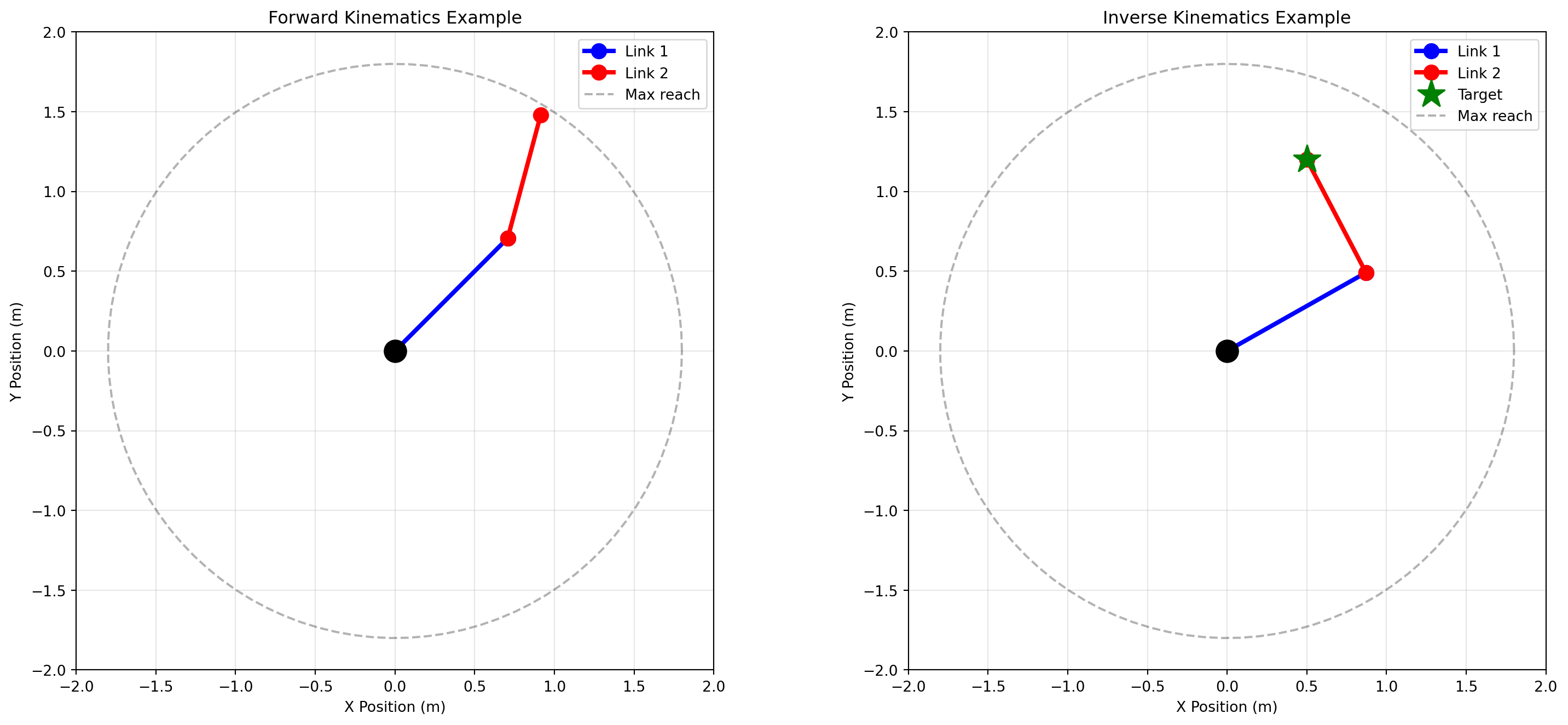
Let’s implement a practical example of robotic control: a 2-DOF (degree-of-freedom) planar robotic arm. We’ll explore both forward kinematics (how joint angles determine end-effector position) and inverse kinematics (how to compute joint angles to reach a target position).

25.6.1 Forward Kinematics

Forward kinematics computes the end-effector position from joint angles. For a 2-link planar arm:

\[ \begin{aligned} x &= l_1 \cos(\theta_1) + l_2 \cos(\theta_1 + \theta_2) \\ y &= l_1 \sin(\theta_1) + l_2 \sin(\theta_1 + \theta_2) \end{aligned} \]

where \(l_1, l_2\) are link lengths and \(\theta_1, \theta_2\) are joint angles.

import numpy as np
import matplotlib.pyplot as plt
from matplotlib.animation import FuncAnimation
from IPython.display import HTML

class PlanarArm2DOF:
    """A 2-DOF planar robotic arm."""

    def __init__(self, l1=1.0, l2=0.8):
        self.l1 = l1  # Length of first link
        self.l2 = l2  # Length of second link

    def forward_kinematics(self, theta1, theta2):
        """Compute end-effector position from joint angles.

        Args:
            theta1: Angle of first joint (radians)
            theta2: Angle of second joint (radians)

        Returns:
            (x, y): End-effector position
        """
        # Position of elbow (end of first link)
        x1 = self.l1 * np.cos(theta1)
        y1 = self.l1 * np.sin(theta1)

        # Position of end-effector
        x2 = x1 + self.l2 * np.cos(theta1 + theta2)
        y2 = y1 + self.l2 * np.sin(theta1 + theta2)

        return (x2, y2), (x1, y1)

    def inverse_kinematics(self, target_x, target_y):
        """Compute joint angles to reach target position.

        Uses analytical solution for 2-DOF planar arm.
        Returns None if target is unreachable.

        Args:
            target_x, target_y: Desired end-effector position

        Returns:
            (theta1, theta2) or None if unreachable
        """
        # Check if target is reachable
        distance = np.sqrt(target_x**2 + target_y**2)
        max_reach = self.l1 + self.l2
        min_reach = abs(self.l1 - self.l2)

        if distance > max_reach or distance < min_reach:
            return None

        # Compute theta2 using law of cosines
        cos_theta2 = (target_x**2 + target_y**2 - self.l1**2 - self.l2**2) / (2 * self.l1 * self.l2)
        cos_theta2 = np.clip(cos_theta2, -1, 1)  # Handle numerical errors

        # Choose elbow-up configuration
        theta2 = np.arccos(cos_theta2)

        # Compute theta1
        k1 = self.l1 + self.l2 * np.cos(theta2)
        k2 = self.l2 * np.sin(theta2)
        theta1 = np.arctan2(target_y, target_x) - np.arctan2(k2, k1)

        return theta1, theta2

    def plot_arm(self, theta1, theta2, target=None, ax=None):
        """Visualize the arm configuration."""
        if ax is None:
            fig, ax = plt.subplots(figsize=(8, 8))

        # Compute positions
        end_pos, elbow_pos = self.forward_kinematics(theta1, theta2)

        # Plot links
        ax.plot([0, elbow_pos[0]], [0, elbow_pos[1]], 'b-o', linewidth=3, markersize=10, label='Link 1')
        ax.plot([elbow_pos[0], end_pos[0]], [elbow_pos[1], end_pos[1]], 'r-o', linewidth=3, markersize=10, label='Link 2')

        # Plot base
        ax.plot(0, 0, 'ko', markersize=15)

        # Plot target if provided
        if target is not None:
            ax.plot(target[0], target[1], 'g*', markersize=20, label='Target')

        # Plot workspace boundary
        theta = np.linspace(0, 2*np.pi, 100)
        max_reach = self.l1 + self.l2
        ax.plot(max_reach * np.cos(theta), max_reach * np.sin(theta), 'k--', alpha=0.3, label='Max reach')

        ax.set_xlim(-2, 2)
        ax.set_ylim(-2, 2)
        ax.set_aspect('equal')
        ax.grid(True, alpha=0.3)
        ax.legend()
        ax.set_xlabel('X Position (m)')
        ax.set_ylabel('Y Position (m)')
        ax.set_title('2-DOF Planar Arm')

        return ax

# Demonstrate forward and inverse kinematics
arm = PlanarArm2DOF(l1=1.0, l2=0.8)

# Forward kinematics example
theta1, theta2 = np.pi/4, np.pi/6
end_pos, _ = arm.forward_kinematics(theta1, theta2)
print(f"Forward kinematics: θ1={np.degrees(theta1):.1f}°, θ2={np.degrees(theta2):.1f}°")
print(f"  → End-effector at ({end_pos[0]:.3f}, {end_pos[1]:.3f})")

# Inverse kinematics example
target = (0.5, 1.2)
result = arm.inverse_kinematics(target[0], target[1])
if result:
    theta1_ik, theta2_ik = result
    print(f" - Inverse kinematics: Target ({target[0]}, {target[1]})")
    print(f"  → θ1={np.degrees(theta1_ik):.1f}°, θ2={np.degrees(theta2_ik):.1f}°")

    # Verify by forward kinematics
    reached_pos, _ = arm.forward_kinematics(theta1_ik, theta2_ik)
    error = np.sqrt((reached_pos[0]-target[0])**2 + (reached_pos[1]-target[1])**2)
    print(f"  → Reached ({reached_pos[0]:.3f}, {reached_pos[1]:.3f}), error: {error:.6f} m")

# Visualize
fig, axes = plt.subplots(1, 2, figsize=(16, 7))

# Plot 1: Forward kinematics
arm.plot_arm(theta1, theta2, ax=axes[0])
axes[0].set_title('Forward Kinematics Example')

# Plot 2: Inverse kinematics
arm.plot_arm(theta1_ik, theta2_ik, target=target, ax=axes[1])
axes[1].set_title('Inverse Kinematics Example')

plt.tight_layout()
plt.show()

Forward kinematics: θ1=45.0°, θ2=30.0°
  → End-effector at (0.914, 1.480)
 - Inverse kinematics: Target (0.5, 1.2)
  → θ1=29.4°, θ2=88.2°
  → Reached (0.500, 1.200), error: 0.000000 m

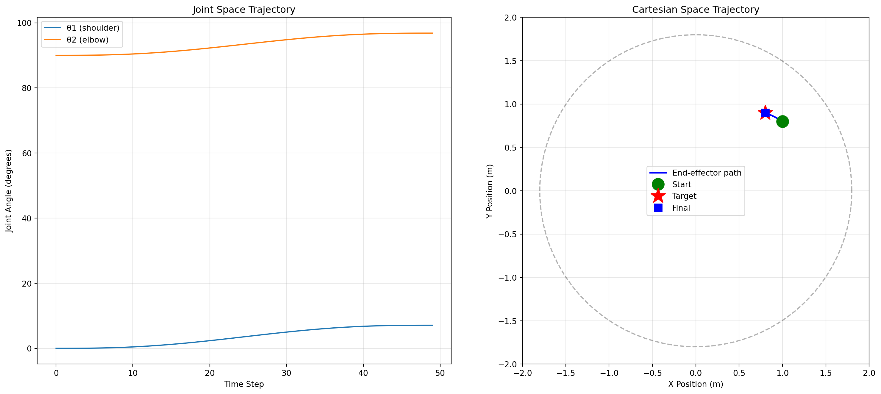
25.6.2 Trajectory Planning and Execution

Reaching a target isn’t just about computing the final joint angles—the arm must move smoothly along a trajectory. We’ll implement a simple trajectory planner that generates smooth joint-space paths.

def plan_trajectory(arm, start_angles, target_pos, num_steps=50):
    """Plan a smooth trajectory to the target.

    Args:
        arm: PlanarArm2DOF instance
        start_angles: (theta1, theta2) starting configuration
        target_pos: (x, y) target position
        num_steps: Number of trajectory steps

    Returns:
        trajectory: List of (theta1, theta2) tuples
    """
    # Compute target angles using inverse kinematics
    target_angles = arm.inverse_kinematics(target_pos[0], target_pos[1])
    if target_angles is None:
        raise ValueError("Target unreachable")

    # Interpolate in joint space using minimum-jerk trajectory
    # This produces smooth, natural-looking movements
    t = np.linspace(0, 1, num_steps)

    # Minimum jerk trajectory (5th order polynomial)
    s = 10 * t**3 - 15 * t**4 + 6 * t**5

    trajectory = []
    for si in s:
        theta1 = start_angles[0] + si * (target_angles[0] - start_angles[0])
        theta2 = start_angles[1] + si * (target_angles[1] - start_angles[1])
        trajectory.append((theta1, theta2))

    return trajectory

# Create a reaching task: move from one position to another
arm = PlanarArm2DOF()
start_angles = (0, np.pi/2)
target_pos = (0.8, 0.9)

# Plan trajectory
trajectory = plan_trajectory(arm, start_angles, target_pos, num_steps=50)

# Visualize trajectory
fig, axes = plt.subplots(1, 2, figsize=(16, 7))

# Left plot: Trajectory in joint space
theta1_traj = [angles[0] for angles in trajectory]
theta2_traj = [angles[1] for angles in trajectory]
axes[0].plot(np.degrees(theta1_traj), label='θ1 (shoulder)')
axes[0].plot(np.degrees(theta2_traj), label='θ2 (elbow)')
axes[0].set_xlabel('Time Step')
axes[0].set_ylabel('Joint Angle (degrees)')
axes[0].set_title('Joint Space Trajectory')
axes[0].legend()
axes[0].grid(True, alpha=0.3)

# Right plot: Trajectory in Cartesian space
end_positions = [arm.forward_kinematics(t[0], t[1])[0] for t in trajectory]
x_traj = [pos[0] for pos in end_positions]
y_traj = [pos[1] for pos in end_positions]

axes[1].plot(x_traj, y_traj, 'b-', linewidth=2, label='End-effector path')
axes[1].plot(x_traj[0], y_traj[0], 'go', markersize=15, label='Start')
axes[1].plot(target_pos[0], target_pos[1], 'r*', markersize=20, label='Target')
axes[1].plot(x_traj[-1], y_traj[-1], 'bs', markersize=10, label='Final')

# Draw workspace
theta = np.linspace(0, 2*np.pi, 100)
max_reach = arm.l1 + arm.l2
axes[1].plot(max_reach * np.cos(theta), max_reach * np.sin(theta), 'k--', alpha=0.3)

axes[1].set_xlim(-2, 2)
axes[1].set_ylim(-2, 2)
axes[1].set_aspect('equal')
axes[1].grid(True, alpha=0.3)
axes[1].legend()
axes[1].set_xlabel('X Position (m)')
axes[1].set_ylabel('Y Position (m)')
axes[1].set_title('Cartesian Space Trajectory')

plt.tight_layout()
plt.show()

print(f"Trajectory length: {len(trajectory)} steps")
print(f"Path length: {np.sum([np.sqrt((x_traj[i+1]-x_traj[i])**2 + (y_traj[i+1]-y_traj[i])**2) for i in range(len(x_traj)-1)]):.3f} m")

Trajectory length: 50 steps
Path length: 0.224 m

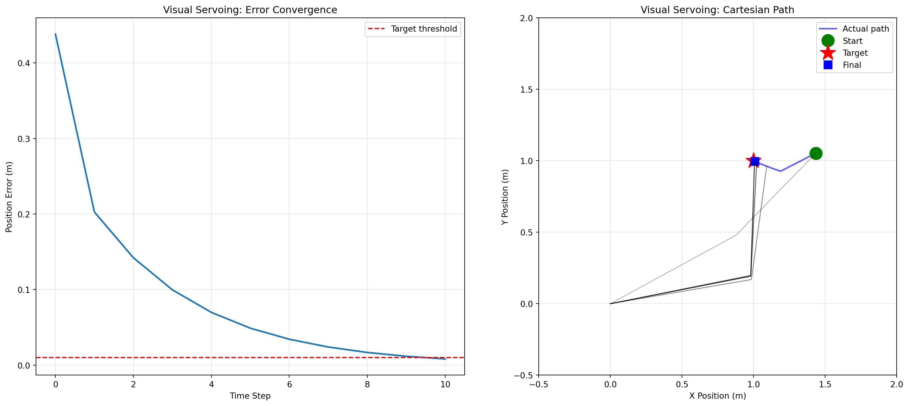
25.6.3 Visual Servoing: Closed-Loop Control

Real robots must deal with uncertainty and errors. Visual servoing uses visual feedback to guide the arm to the target, correcting for errors in real-time—analogous to how your visual cortex guides your hand when reaching for a cup.

def visual_servoing(arm, start_angles, target_pos, num_steps=100, gain=0.1):
    """Control arm to target using visual feedback.

    Implements proportional control: at each step, move toward
    the target proportional to the current error.

    Args:
        arm: PlanarArm2DOF instance
        start_angles: Starting configuration
        target_pos: Target position
        num_steps: Maximum number of control steps
        gain: Proportional control gain

    Returns:
        trajectory: List of (theta1, theta2) tuples
        errors: List of position errors
    """
    trajectory = [start_angles]
    errors = []

    theta1, theta2 = start_angles

    for step in range(num_steps):
        # Get current end-effector position (vision)
        current_pos, _ = arm.forward_kinematics(theta1, theta2)

        # Compute error
        error_x = target_pos[0] - current_pos[0]
        error_y = target_pos[1] - current_pos[1]
        error_magnitude = np.sqrt(error_x**2 + error_y**2)
        errors.append(error_magnitude)

        # Check if reached target
        if error_magnitude < 0.01:
            break

        # Compute Jacobian (maps joint velocities to end-effector velocities)
        J = np.array([
            [-arm.l1*np.sin(theta1) - arm.l2*np.sin(theta1+theta2), -arm.l2*np.sin(theta1+theta2)],
            [arm.l1*np.cos(theta1) + arm.l2*np.cos(theta1+theta2), arm.l2*np.cos(theta1+theta2)]
        ])

        # Compute desired end-effector velocity (proportional control)
        desired_vel = gain * np.array([error_x, error_y])

        # Compute joint velocities using pseudo-inverse of Jacobian
        J_pinv = np.linalg.pinv(J)
        joint_vel = J_pinv @ desired_vel

        # Update joint angles
        theta1 += joint_vel[0]
        theta2 += joint_vel[1]

        trajectory.append((theta1, theta2))

    return trajectory, errors

# Test visual servoing with a perturbation
start_angles = (0.5, 0.3)
target_pos = (1.0, 1.0)

trajectory_vs, errors_vs = visual_servoing(arm, start_angles, target_pos, num_steps=100, gain=0.3)

# Visualize results
fig, axes = plt.subplots(1, 2, figsize=(16, 7))

# Left: Convergence plot
axes[0].plot(errors_vs, linewidth=2)
axes[0].set_xlabel('Time Step')
axes[0].set_ylabel('Position Error (m)')
axes[0].set_title('Visual Servoing: Error Convergence')
axes[0].grid(True, alpha=0.3)
axes[0].axhline(y=0.01, color='r', linestyle='--', label='Target threshold')
axes[0].legend()

# Right: Trajectory in Cartesian space
end_positions_vs = [arm.forward_kinematics(t[0], t[1])[0] for t in trajectory_vs]
x_traj_vs = [pos[0] for pos in end_positions_vs]
y_traj_vs = [pos[1] for pos in end_positions_vs]

axes[1].plot(x_traj_vs, y_traj_vs, 'b-', linewidth=2, alpha=0.6, label='Actual path')
axes[1].plot(x_traj_vs[0], y_traj_vs[0], 'go', markersize=15, label='Start')
axes[1].plot(target_pos[0], target_pos[1], 'r*', markersize=20, label='Target')
axes[1].plot(x_traj_vs[-1], y_traj_vs[-1], 'bs', markersize=10, label='Final')

# Draw arm at several time points
sample_indices = [0, len(trajectory_vs)//3, 2*len(trajectory_vs)//3, -1]
for i, idx in enumerate(sample_indices):
    theta1, theta2 = trajectory_vs[idx]
    end_pos, elbow_pos = arm.forward_kinematics(theta1, theta2)
    alpha = 0.3 + 0.7 * (i / len(sample_indices))
    axes[1].plot([0, elbow_pos[0], end_pos[0]], [0, elbow_pos[1], end_pos[1]],
                'k-', alpha=alpha, linewidth=1)

axes[1].set_xlim(-0.5, 2)
axes[1].set_ylim(-0.5, 2)
axes[1].set_aspect('equal')
axes[1].grid(True, alpha=0.3)
axes[1].legend()
axes[1].set_xlabel('X Position (m)')
axes[1].set_ylabel('Y Position (m)')
axes[1].set_title('Visual Servoing: Cartesian Path')

plt.tight_layout()
plt.show()

print(f"Visual servoing converged in {len(trajectory_vs)} steps")
print(f"Final error: {errors_vs[-1]:.6f} m")

Visual servoing converged in 11 steps
Final error: 0.008245 m

This code lab demonstrates key principles of robotic control:

• Forward/Inverse Kinematics: The fundamental transformations between joint and Cartesian spaces.
• Trajectory Planning: Generating smooth, natural movements (analogous to motor planning in premotor cortex).
• Visual Servoing: Closed-loop control using sensory feedback (analogous to visual-motor integration in parietal cortex).

The visual servoing approach is particularly brain-inspired: rather than planning the entire trajectory upfront, the controller continuously adjusts based on current sensory information—just like your brain does when reaching for a moving target.

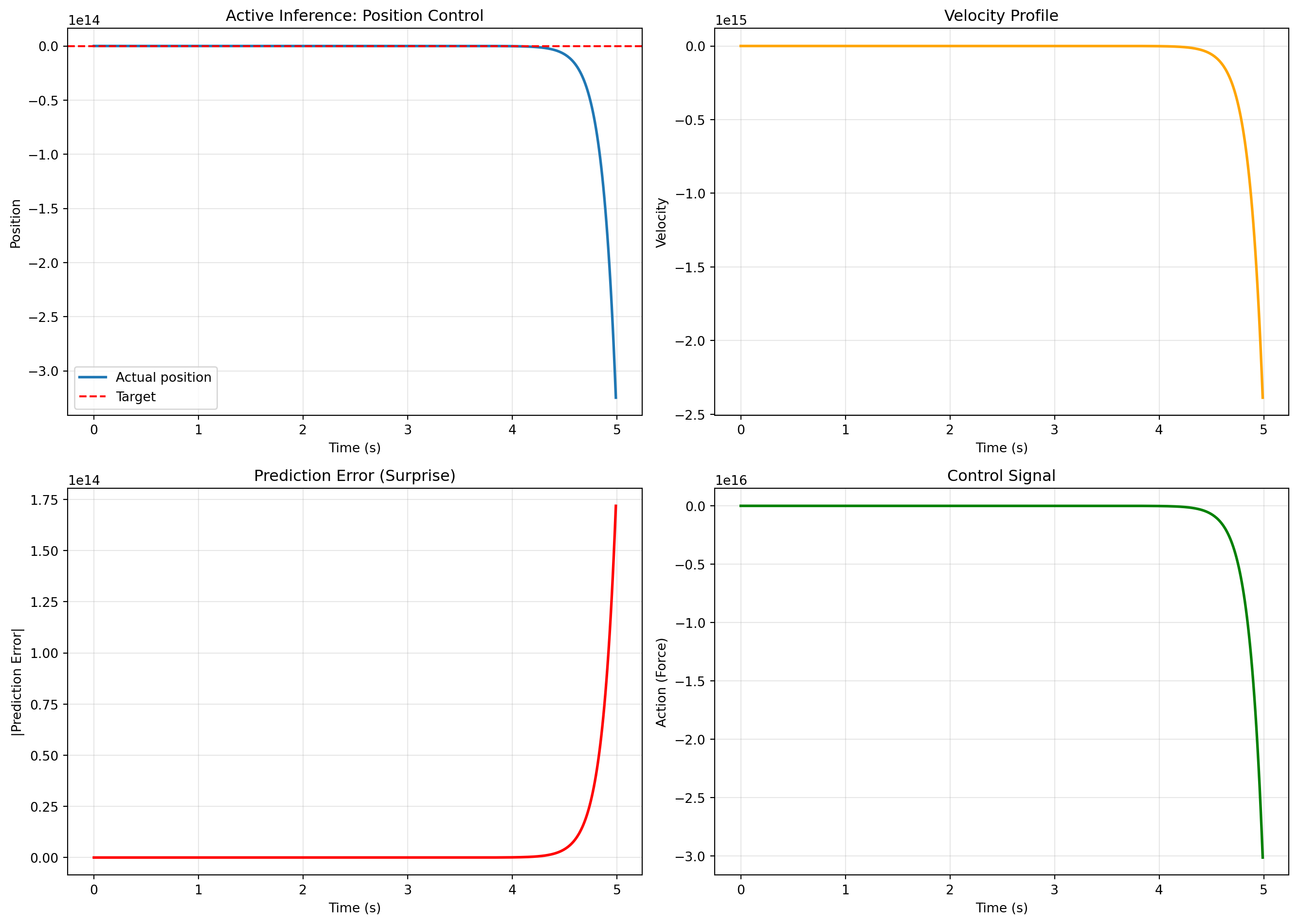
35.7 25.7 Code Lab: Active Inference for Sensorimotor Control

Active inference is a neuroscience-inspired framework that unifies perception, action, and learning under a single principle: minimizing surprise (or equivalently, minimizing free energy). Unlike traditional control approaches that separate perception and action, active inference views both as strategies for minimizing prediction errors.

25.7.1 The Free Energy Principle

The core idea: the brain maintains an internal model of the world and constantly generates predictions about sensory inputs. When there’s a mismatch between prediction and reality, the brain has two options:

1. Perceptual inference: Update beliefs about the world to better explain the sensory input.
2. Active inference: Perform actions to change the sensory input to match predictions.

Both strategies minimize free energy, an information-theoretic quantity that bounds surprise. Mathematically:

\[ F = E_q[\log q(s) - \log p(o, s)] = D_{KL}[q(s)||p(s|o)] - \log p(o) \]

where \(o\) is observations, \(s\) is hidden states, \(q(s)\) is the agent’s beliefs, and \(p(s|o)\) is the true posterior.

25.7.2 Implementing a Simple Active Inference Agent

We’ll implement an active inference agent controlling a 1-DOF system (a single joint) reaching for a target. The agent has:

• Generative model: A belief about how its actions affect sensory input.
• Prediction errors: Mismatches between predicted and actual sensations.
• Action policy: Actions that minimize expected free energy.

class ActiveInferenceAgent:
    """A simple active inference agent for 1-DOF control."""

    def __init__(self, target_position, dt=0.01):
        """
        Args:
            target_position: Desired position (agent's prior belief)
            dt: Time step
        """
        self.target_position = target_position
        self.dt = dt

        # Current state
        self.position = 0.0
        self.velocity = 0.0

        # Sensory prediction parameters
        self.predicted_position = target_position
        self.predicted_velocity = 0.0

        # Precision (inverse variance) of predictions
        # High precision = strong belief
        self.precision_position = 10.0
        self.precision_velocity = 5.0
        self.precision_action = 0.5

        # History
        self.history = {
            'time': [],
            'position': [],
            'velocity': [],
            'prediction_error': [],
            'action': []
        }

    def sensory_prediction_error(self):
        """Compute prediction errors (predicted - actual)."""
        error_position = self.predicted_position - self.position
        error_velocity = self.predicted_velocity - self.velocity
        return error_position, error_velocity

    def compute_action(self):
        """Compute action that minimizes free energy.

        Action is chosen to bring sensory input closer to predictions.
        This implements the reflex arc: prediction error → action.
        """
        error_pos, error_vel = self.sensory_prediction_error()

        # Action is proportional to weighted prediction errors
        # (weights = precisions = inverse variances)
        action = (self.precision_position * error_pos +
                  self.precision_velocity * error_vel)

        # Action cost (prevents overly large actions)
        action = action / (1 + self.precision_action)

        return action

    def update_beliefs(self):
        """Update predictions based on current state (perceptual inference).

        In this simple implementation, we use gradient descent on free energy.
        """
        error_pos, error_vel = self.sensory_prediction_error()

        # Update predicted velocity toward actual velocity
        self.predicted_velocity += 0.1 * error_vel

        # Predicted position is pulled toward prior (target) and current observation
        prior_pull = 0.05 * (self.target_position - self.predicted_position)
        evidence_pull = 0.1 * error_pos
        self.predicted_position += prior_pull - evidence_pull

    def step(self, action):
        """Execute action and update internal state."""
        # Simple physics: acceleration = action
        acceleration = action
        self.velocity += acceleration * self.dt

        # Add damping
        self.velocity *= 0.95

        self.position += self.velocity * self.dt

        # Update beliefs (perceptual inference)
        self.update_beliefs()

        # Record history
        error_pos, _ = self.sensory_prediction_error()
        self.history['time'].append(len(self.history['time']) * self.dt)
        self.history['position'].append(self.position)
        self.history['velocity'].append(self.velocity)
        self.history['prediction_error'].append(abs(error_pos))
        self.history['action'].append(action)

# Run active inference agent
agent = ActiveInferenceAgent(target_position=1.0, dt=0.01)

for step in range(500):
    action = agent.compute_action()
    agent.step(action)

# Visualize results
fig, axes = plt.subplots(2, 2, figsize=(14, 10))

# Position over time
axes[0, 0].plot(agent.history['time'], agent.history['position'], label='Actual position', linewidth=2)
axes[0, 0].axhline(y=agent.target_position, color='r', linestyle='--', label='Target')
axes[0, 0].set_xlabel('Time (s)')
axes[0, 0].set_ylabel('Position')
axes[0, 0].set_title('Active Inference: Position Control')
axes[0, 0].legend()
axes[0, 0].grid(True, alpha=0.3)

# Velocity over time
axes[0, 1].plot(agent.history['time'], agent.history['velocity'], color='orange', linewidth=2)
axes[0, 1].set_xlabel('Time (s)')
axes[0, 1].set_ylabel('Velocity')
axes[0, 1].set_title('Velocity Profile')
axes[0, 1].grid(True, alpha=0.3)

# Prediction error over time
axes[1, 0].plot(agent.history['time'], agent.history['prediction_error'], color='red', linewidth=2)
axes[1, 0].set_xlabel('Time (s)')
axes[1, 0].set_ylabel('|Prediction Error|')
axes[1, 0].set_title('Prediction Error (Surprise)')
axes[1, 0].grid(True, alpha=0.3)

# Action over time
axes[1, 1].plot(agent.history['time'], agent.history['action'], color='green', linewidth=2)
axes[1, 1].set_xlabel('Time (s)')
axes[1, 1].set_ylabel('Action (Force)')
axes[1, 1].set_title('Control Signal')
axes[1, 1].grid(True, alpha=0.3)

plt.tight_layout()
plt.show()

print(f"Final position: {agent.history['position'][-1]:.4f}")
print(f"Target position: {agent.target_position}")
print(f"Final error: {abs(agent.history['position'][-1] - agent.target_position):.4f}")

Final position: -324705659140302.8750
Target position: 1.0
Final error: 324705659140303.8750

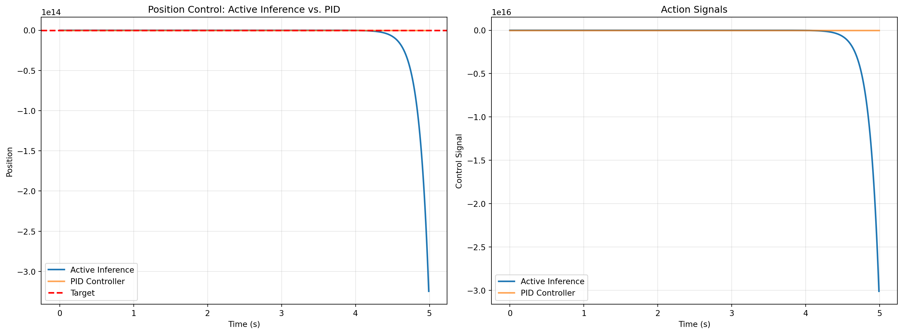
25.7.3 Comparison to Traditional Control

Let’s compare active inference to a traditional PID controller to highlight the conceptual differences.

class PIDController:
    """Traditional PID controller for comparison."""

    def __init__(self, target, kp=2.0, ki=0.1, kd=1.0, dt=0.01):
        self.target = target
        self.kp = kp  # Proportional gain
        self.ki = ki  # Integral gain
        self.kd = kd  # Derivative gain
        self.dt = dt

        self.position = 0.0
        self.velocity = 0.0
        self.integral_error = 0.0
        self.prev_error = 0.0

        self.history = {
            'time': [],
            'position': [],
            'action': []
        }

    def compute_action(self):
        """Compute PID control signal."""
        error = self.target - self.position
        self.integral_error += error * self.dt
        derivative_error = (error - self.prev_error) / self.dt

        action = (self.kp * error +
                  self.ki * self.integral_error +
                  self.kd * derivative_error)

        self.prev_error = error
        return action

    def step(self, action):
        """Execute action and update state."""
        acceleration = action
        self.velocity += acceleration * self.dt
        self.velocity *= 0.95  # Damping
        self.position += self.velocity * self.dt

        self.history['time'].append(len(self.history['time']) * self.dt)
        self.history['position'].append(self.position)
        self.history['action'].append(action)

# Run PID controller
pid = PIDController(target=1.0, dt=0.01)

for step in range(500):
    action = pid.compute_action()
    pid.step(action)

# Compare both controllers
fig, axes = plt.subplots(1, 2, figsize=(16, 6))

# Position comparison
axes[0].plot(agent.history['time'], agent.history['position'],
             label='Active Inference', linewidth=2)
axes[0].plot(pid.history['time'], pid.history['position'],
             label='PID Controller', linewidth=2, alpha=0.7)
axes[0].axhline(y=1.0, color='r', linestyle='--', label='Target', linewidth=2)
axes[0].set_xlabel('Time (s)')
axes[0].set_ylabel('Position')
axes[0].set_title('Position Control: Active Inference vs. PID')
axes[0].legend()
axes[0].grid(True, alpha=0.3)

# Action comparison
axes[1].plot(agent.history['time'], agent.history['action'],
             label='Active Inference', linewidth=2)
axes[1].plot(pid.history['time'], pid.history['action'],
             label='PID Controller', linewidth=2, alpha=0.7)
axes[1].set_xlabel('Time (s)')
axes[1].set_ylabel('Control Signal')
axes[1].set_title('Action Signals')
axes[1].legend()
axes[1].grid(True, alpha=0.3)

plt.tight_layout()
plt.show()

print(); print("=== Performance Comparison ===")
print(f"Active Inference - Final error: {abs(agent.history['position'][-1] - 1.0):.4f}")
print(f"PID Controller - Final error: {abs(pid.history['position'][-1] - 1.0):.4f}")
print(f" - Active Inference - Action variance: {np.var(agent.history['action']):.4f}")
print(f"PID Controller - Action variance: {np.var(pid.history['action']):.4f}")

=== Performance Comparison ===
Active Inference - Final error: 324705659140303.8750
PID Controller - Final error: 0.1003
 - Active Inference - Action variance: 12136832984926238099205636751360.0000
PID Controller - Action variance: 20.5459

Key Insights:

• Active Inference: Control emerges from the drive to minimize prediction error. The agent acts to make the world match its predictions (which are biased toward the target).
• PID Control: Explicit error-correction based on current, accumulated, and predicted future error.
• Biological Plausibility: Active inference maps more naturally onto neural circuits. Prediction errors could be represented by neural firing rates, and action selection could be implemented by population codes in motor cortex.
• Adaptability: Active inference can naturally incorporate uncertainty (via precisions), making it more robust to sensory noise and better at handling ambiguous situations.

This framework suggests that motor control in the brain may not be fundamentally about computing error-correction signals, but about maintaining predictions and acting to fulfill them—a profound reconceptualization that places prediction at the heart of both perception and action.

35.8 25.8 Learning Like Infants: Developmental Robotics

Human infants are arguably the most capable learning systems on Earth. With minimal supervision and no explicit training signal, they master perception, manipulation, locomotion, and language within just a few years. Developmental robotics seeks to understand and replicate this learning process in machines.

25.8.1 Stages of Sensorimotor Development

Infant development follows a remarkably consistent trajectory across cultures, suggesting it reflects fundamental principles of embodied learning:

Stage 1: Reflexes and Random Exploration (0-1 months) - Infants begin with basic reflexes (grasping, sucking, startle response). - Random motor babbling generates diverse sensorimotor experiences. - The brain begins building associations: When I move my arm this way, I see my hand move like that.

Stage 2: Primary Circular Reactions (1-4 months) - Infants discover they can produce interesting sensory effects through actions. - Repeating actions that produce pleasing results (kicking a mobile, watching hands). - Emergence of simple sensorimotor schemas: action-effect mappings.

Stage 3: Secondary Circular Reactions (4-8 months) - Focus shifts from self to external objects. - Infants learn they can affect the world (shaking a rattle produces sound). - Beginning of intentional action: acting in order to produce an effect.

Stage 4: Coordination of Schemas (8-12 months) - Multiple action schemes combine to achieve goals. - Object permanence: understanding that objects continue to exist when hidden. - Means-end reasoning: using one action as a means to enable another.

Stage 5: Tertiary Circular Reactions (12-18 months) - Systematic experimentation: varying actions to discover new effects. - True exploration: “What happens if I drop this from different heights?” - Scientific thinking emerges from embodied exploration.

Stage 6: Mental Representation (18+ months) - Internal simulation of actions before executing them. - Symbolic thought and deferred imitation. - Language learning accelerates as symbols become grounded in sensorimotor experience.

25.8.2 Curiosity-Driven Exploration

A key insight from developmental psychology: infants are not passively absorbing information—they are actively seeking it. They are intrinsically motivated to explore, driven by curiosity.

Computational models of curiosity define it as seeking situations where learning progress is maximized. An infant doesn’t repeatedly shake a rattle for hours (already learned), nor try to solve calculus problems (impossible to learn currently). Instead, infants seek the “Goldilocks zone”—tasks that are challenging but learnable.

This can be formalized as maximizing learning progress:

\[ \text{Curiosity}(s) = |L_t(s) - L_{t-\Delta t}(s)| \]

where \(L_t(s)\) is the prediction error in situation \(s\) at time \(t\). High curiosity corresponds to situations where prediction error is decreasing rapidly—learning is happening.

In developmental robotics, this principle can guide exploration:

class CuriousBaby Robot:
    def choose_next_action(self):
        # For each possible action:
        for action in self.action_space:
            # Estimate how much learning progress it would produce
            predicted_learning = self.estimate_learning_progress(action)

        # Choose action with highest predicted learning
        return argmax(predicted_learning)

This simple principle leads to complex, structured behavior. Early in development, the robot explores its own body (moving joints, observing effects). Once body control is mastered (learning progress plateaus), curiosity drives the robot to interact with objects. Once simple object interactions are mastered, curiosity drives exploration of multi-object interactions and tool use.

25.8.3 Object Permanence and Affordance Learning

One of the most significant developmental milestones is object permanence—the understanding that objects continue to exist even when not perceived. This requires building persistent internal representations.

A robot can develop object permanence through embodied interaction:

1. Phase 1: Objects only “exist” when visible. When an object moves behind an occluder, the robot treats it as disappeared.
2. Phase 2: Through repeated experience (objects reappearing from behind occluders), the robot learns to predict “If object moved left behind occluder, it will likely reappear on the left side.”
3. Phase 3: The robot builds full spatiotemporal models: maintaining representations of object position and motion even during occlusion.

Simultaneously, robots learn affordances—what actions are possible with objects:

• Graspable: Objects of certain sizes and shapes can be grasped.
• Pushable: Objects slide when pushed (but not walls).
• Stackable: Flat-topped objects support other objects.
• Rollable: Circular objects behave differently from cubes.

These affordances are not explicitly programmed—they emerge from sensorimotor experience. A robot that repeatedly pushes objects learns to predict “If I push this object-type, it moves this way.” This prediction is an affordance.

25.8.4 Curriculum Learning from Embodiment

The stages of infant development form a natural curriculum—a sequence of increasingly complex tasks. This is not engineered by a teacher; it emerges from the statistics of embodied interaction.

Why this order?

• Body before world: Learning body control is simpler (more predictable) than learning about external objects. Embodiment naturally creates a curriculum that starts with the easier problem.
• Near before far: Infants first master reaching for nearby objects before coordinating across larger distances. The physics of nearby interaction are simpler (less affected by arm dynamics).
• Static before dynamic: Grasping stationary objects precedes catching moving objects. Static tasks are more predictable.
• Single before multiple: Interacting with one object precedes multi-object reasoning. Fewer variables to track.

This suggests a design principle for robot learning: Don’t specify the curriculum; let it emerge from embodiment and curiosity. The robot’s body, sensors, and environment naturally constrain the space of possible experiences in a way that scaffolds learning.

25.8.5 The Role of Play in Skill Acquisition

Human children spend enormous amounts of time playing—activities with no immediate goal beyond the activity itself. This seems wasteful from an engineering perspective, but developmental robotics suggests play is a critical learning mechanism.

Play as exploration of possibilities: When a child builds a tower of blocks and then knocks it down, they’re learning about: - Gravity and stability - Object properties (some blocks stack better than others) - Cause and effect (my action causes tower to fall) - Planning (how high can I build before it falls?)

Play as skill composition: Children combine mastered skills in novel ways during play, creating a library of reusable action sequences. This is exactly what hierarchical reinforcement learning attempts to achieve through “options” and “skills.”

Play as safe learning: Play provides a low-stakes environment to learn. Failures during play have no negative consequences, allowing aggressive exploration. This mirrors “curiosity-driven learning” in AI—the intrinsic reward for exploration enables learning without external rewards.

Developmental robotics systems that incorporate play behaviors show accelerated learning and better transfer to novel tasks. The robot that “plays” with objects (manipulating them in varied ways with no specific goal) later performs goal-directed manipulation tasks more successfully than a robot trained only on the target task.

35.9 25.9 Predictive Processing and Motor Control

The brain is fundamentally a prediction machine. The predictive processing framework proposes that every level of the neural hierarchy is constantly generating predictions about the level below, and only prediction errors—surprises—propagate upward. This has profound implications for understanding motor control.

25.9.1 Forward Models and Efference Copy

When you decide to move your arm, your motor cortex sends motor commands to your spinal cord. But simultaneously, it sends a copy of this command—called an efference copy or corollary discharge—to the cerebellum and sensory cortex. This copy is used to predict the sensory consequences of the movement.

This creates two parallel streams:

1. Motor command → Muscles → Actual sensory feedback
2. Efference copy → Forward model → Predicted sensory feedback

By comparing predicted and actual feedback, the brain can:

• Distinguish self from world: If you touch your arm with your finger, the sensory cortex predicts the touch (from the efference copy), so it feels less intense than if someone else touches you.
• Cancel out self-generated sensations: This is why you can’t tickle yourself—your cerebellum predicts the sensation, and the predicted sensation is subtracted from the actual sensation.
• Detect errors: Any mismatch between predicted and actual feedback indicates something unexpected happened (e.g., your hand hit an obstacle).

Mathematically, this can be represented as:

\[ \text{Prediction Error} = \text{Actual Sensory Feedback} - \text{Forward Model}(\text{Efference Copy}) \]

25.9.2 Minimizing Prediction Error: Two Strategies

When prediction error occurs, the brain has two strategies to reduce it:

Strategy 1: Update the forward model (Perceptual Learning) - If prediction errors are consistent, the cerebellum updates its forward model. - Example: When you first put on a heavy backpack, your movements feel off. Quickly, your cerebellum adapts its forward model to account for the added mass. - This is motor adaptation—learning new sensorimotor mappings.

Strategy 2: Change your actions (Motor Correction) - If prediction error indicates your action isn’t achieving its goal, issue corrective motor commands. - Example: Your hand is reaching toward a cup, but visual feedback shows it’s veering left. You generate a correction to move right. - This is online motor correction—real-time adjustment of ongoing movements.

These aren’t distinct mechanisms—they operate simultaneously at multiple timescales. Fast corrections happen in milliseconds (spinal reflexes), medium corrections in tens of milliseconds (cerebellar corrections), and slow corrections via cortical replanning (hundreds of milliseconds).

25.9.3 The Cerebellum as a Forward Model

The cerebellum is ideally structured to learn forward models:

• Inputs: Motor commands (from motor cortex) and current state (proprioception, vision).
• Output: Predicted sensory consequences.
• Learning signal: Prediction errors (actual sensory feedback - predicted feedback).

Neurophysiological evidence supports this:

• Purkinje cells in the cerebellum show firing patterns that precede movements, consistent with generating predictions.
• Climbing fiber inputs carry error signals that trigger synaptic plasticity.
• Cerebellar lesions impair motor timing and coordination, consistent with loss of forward model prediction.

Computational models show that training a neural network with cerebellar-like architecture to predict sensory consequences of actions enables smooth, coordinated movement. The network learns the physics of the body implicitly through sensorimotor experience.

25.9.4 Connection to Optimal Control Theory

Predictive processing connects to classical control theory through Model Predictive Control (MPC). MPC works by:

1. Using a forward model to simulate future trajectories for different action sequences.
2. Selecting the action sequence that minimizes a cost function (e.g., energy expenditure, time to goal).
3. Executing the first action in the sequence.
4. Repeating the process (receding horizon control).

This is essentially what the brain does:

• Forward model: Cerebellum predicts consequences of motor commands.
• Cost function: Encoded in basal ganglia and prefrontal cortex (reward, effort, goal proximity).
• Optimization: Motor cortex and premotor areas select actions that minimize predicted cost.
• Receding horizon: Plans are constantly updated as new sensory information arrives.

The key insight: optimal control emerges from prediction and prediction error minimization. You don’t need an explicit optimization algorithm—a neural network that learns to predict and act to minimize prediction error will exhibit near-optimal behavior.

This provides a unified framework connecting:

• Neuroscience: Cerebellar forward models, motor cortex planning, sensory prediction errors.
• Robotics: Model predictive control, adaptive control, learning-based control.
• Machine learning: Predictive models, world models, model-based reinforcement learning.

All are different perspectives on the same core principle: intelligent behavior arises from prediction.

35.10 25.10 The Body as a Tool: Brain-Inspired Motor Control

Controlling a physical body is a problem of incredible complexity. The brain must coordinate hundreds of muscles to produce smooth, precise movements. It does so not by micromanaging every muscle fiber, but by using clever, hierarchical strategies that robotics is now beginning to emulate.

25.10.1 Motor Primitives: The “Chords” of Movement

A pianist doesn’t think about the individual muscles in their fingers. They think in terms of chords and scales—motor primitives. These are reusable, coordinated patterns of muscle activation. The brain learns a vocabulary of these primitives and then composes them to create a limitless variety of complex movements.

In robotics, this approach simplifies control dramatically. Instead of learning a policy over hundreds of individual motors, the AI learns a policy over a small set of useful primitives (e.g., “reach,” “grasp,” “lift”).

25.10.2 Forward Models: Thinking Before You Act

When you reach to catch a ball, your brain doesn’t just react to what it sees. It runs a fast, internal simulation—a forward model—that predicts the trajectory of the ball and the sensory consequences of your own arm movement. This allows you to move your hand to where the ball will be, not where it was.

This predictive control is a key function of the cerebellum. In robotics, forward models are used to: - Plan Actions: By simulating the outcome of different motor commands, the robot can choose the one that best achieves its goal. - Adapt on the Fly: By comparing the predicted sensory feedback to the actual feedback, the robot can detect errors and make rapid corrections.

The Bike Riding Analogy Learning to ride a bike is a perfect example of embodied learning. - You start with basic motor primitives (pedaling, steering). - Your cerebellum learns a forward model: “If I lean this much and turn the handlebars this much, I will feel myself tipping over.” - You learn from prediction errors: The feeling of falling is a massive error signal that tells your cerebellum its forward model was wrong, forcing it to adapt. - Eventually, the forward model becomes so accurate that you can balance and steer without conscious thought. You have embodied the skill.

35.11 25.11 The Body as a Lens: Action-Centered Perception

Embodiment doesn’t just change how an agent acts; it changes how it perceives. The brain’s perceptual systems are not designed to create a perfect, objective reconstruction of the world. They are designed to answer the question, “What can I do here?”

This is the theory of affordances. We don’t just see a chair; we see a “sittable” object. We don’t just see a cup; we see a “graspable,” “liftable,” “drinkable-from” object. Our perception of the world is fundamentally action-centered.

In robotics, this principle is used to simplify perception. Instead of trying to identify every object in a scene, an affordance-based system directly looks for action possibilities. A robot looking for a tool doesn’t need to recognize a “hammer”; it needs to find an object with the affordance of “hammerable-with” (e.g., something with a long handle and a heavy head). This makes perception more efficient and directly relevant to the agent’s goals.

Neuroscience Connection: The parietal cortex in the brain is thought to be a key hub for affordance perception, transforming visual information about objects into representations of potential actions.

35.12 25.12 The Body Among Others: Social Robotics

Having a body means sharing a physical space with other embodied agents, most notably humans. Social robotics is the field of designing robots that can interact and collaborate with people safely and intuitively. This requires a whole new set of brain-inspired capabilities.

• Joint Attention: The ability to follow a person’s gaze or pointing gesture to share a common focus of attention. This is a foundational skill for learning and collaboration, rooted in the brain’s social cognition networks.
• Intent Prediction: A robot must be able to predict a human’s intentions from their movements and actions to be a helpful partner. If a person reaches for a cabinet, the robot should infer they intend to get a cup and might move to assist.
• Learning from Demonstration: Instead of being explicitly programmed, social robots can learn new skills by watching a human perform them, tapping into neural mechanisms related to the brain’s mirror neuron system.

The ultimate goal is to create robots that are not just tools, but true collaborators, seamlessly integrating into human environments because they understand the unwritten rules of physical and social interaction.

Chapter Summary This chapter argued for the Embodiment Hypothesis: the idea that a physical body is not an optional accessory for intelligence, but a fundamental requirement.

• The Body as a Teacher: We saw how the sensorimotor loop of acting and sensing provides the grounded, self-supervised data necessary for an agent to learn about the physical world.
• Real-World Case Studies: We examined how modern robotics systems from Boston Dynamics use Central Pattern Generators for locomotion, how soft robotics exploits morphological computation, and how sim-to-real transfer with domain randomization enables learning in simulation to transfer to physical robots.
• Hands-On Implementation: Through code labs, we implemented inverse kinematics for robotic arm control, visual servoing for closed-loop feedback, and active inference as an alternative to traditional PID control.
• Developmental Robotics: We explored how robots can learn like infants through curiosity-driven exploration, progressing through natural stages of sensorimotor development, learning object permanence and affordances through embodied interaction.
• Predictive Processing: We unified motor control under the framework of prediction and prediction error minimization, connecting neuroscience (cerebellar forward models), robotics (model predictive control), and optimal control theory.
• The Body as a Tool: We explored how the brain controls a complex body using efficient strategies like motor primitives and predictive forward models, principles that are now central to modern robotics.
• The Body as a Lens: We reframed perception as being action-centered through the concept of affordances, where an agent perceives the world in terms of the actions it can perform.
• The Body Among Others: We examined the challenges of social robotics, where embodied agents must learn to interact, collaborate, and learn from humans, drawing on the brain’s social cognition abilities.

Ultimately, the path to more general and robust AI may not be through bigger datasets and larger models alone, but through getting our AI out of the digital “vat” and into the real world.

Knowledge Connections Looking Back - Chapter 6 (Motor Systems): The biological motor control systems discussed there, particularly the cerebellum and basal ganglia, are the direct inspiration for the forward models and reinforcement learning techniques used in modern robotics. - Chapter 17 (BCIs): Brain-Computer Interfaces represent the ultimate fusion of mind and machine, providing a direct control path from the brain’s motor cortex to the robotic actuators discussed in this chapter.

Looking Forward - Chapter 23 (Lifelong Learning): The ability of an embodied agent to learn continuously from its stream of sensorimotor experience is a core challenge of lifelong learning.

35.13 Exercises

Conceptual Questions

1. Explain the Embodiment Hypothesis and its implications for AI. Why might a “brain in a vat” be fundamentally limited in developing general intelligence? Provide examples of concepts or skills that might require physical interaction with the world to truly understand.

2. Compare motor primitives in biology and robotics. Describe how the brain uses motor primitives (coordinated muscle activation patterns) to simplify control. How is this principle implemented in robotic systems? What are the advantages of a primitives-based approach over direct motor control?

3. Explain the role of forward models in motor control. What is a forward model, and how does the cerebellum use it for predictive control? How are forward models used in robotics for planning and error correction? Provide a concrete example (e.g., catching a ball, reaching for an object).

4. Describe affordance-based perception. How does the concept of affordances reframe perception as action-centered? Compare this to traditional object recognition in computer vision. How might affordance-based perception make robotic systems more efficient and goal-directed?

Computational Exercises

5. Implement a simple sensorimotor learning loop. Create:
   • A simulated agent in a gridworld environment
   • Implement the sense-act-learn loop
   • Have the agent learn to predict the consequences of its actions
   • Build an internal model: action → state change
   • Test the agent’s ability to plan using its learned model
   • Compare to model-free learning (no internal model)
6. Simulate motor primitive composition. Implement:
   • A set of basic motor primitives (e.g., reach, grasp, lift, place)
   • A mechanism to sequence and blend primitives
   • Train the system to perform a composite task (e.g., pick and place)
   • Compare learning time and performance to learning the full task end-to-end
   • Visualize the primitive activations during task execution
7. Build a simple forward model. Create:
   • A simulated robot arm reaching task
   • Train a neural network as a forward model: (state, action) → predicted next state
   • Use the forward model to plan trajectories via model predictive control
   • Compare planning quality with accurate vs. inaccurate forward models
   • Demonstrate error correction when the forward model prediction differs from reality
8. Implement affordance detection. Implement:
   • A vision system that detects affordances rather than objects
   • For a robotic manipulation task, identify “graspable” regions in images
   • Compare affordance-based vs. object-recognition-based approaches
   • Measure task success rate for each method
   • Discuss generalization to novel objects

Discussion Questions

9. The importance of embodiment for different AI capabilities. Discuss:
   • Which AI capabilities fundamentally require embodiment (physical grounding)?
   • Can large language models develop genuine understanding of physical concepts without embodiment?
   • How might simulation environments partially satisfy embodiment requirements?
   • What is the “sim-to-real gap,” and how does it limit the transfer of embodied learning?
10. Social robotics and human-robot collaboration. Consider:
    • What makes human-human collaboration so seamless (joint attention, intent prediction, implicit communication)?
    • How can robots learn to predict human intentions from movement and gaze?
    • What role does the mirror neuron system play in learning from demonstration?
    • What are the key challenges in making robots safe and trustworthy collaborators?
11. Embodied cognition and the future of AI. Reflect on:
    • Could embodied AI agents develop emergent capabilities that disembodied models cannot?
    • How might combining large language models with robotic embodiment create more capable systems?
    • What are the practical barriers to scaling embodied AI (cost, safety, complexity)?
    • How should research priorities balance scaling disembodied models vs. developing embodied systems?

35.14 References

Case Studies and Robotics Systems

Raibert, M., Blankespoor, K., Nelson, G., & Playter, R. (2008). Bigdog, the rough-terrain quadruped robot. IFAC Proceedings Volumes, 41(2), 10822-10825.

Kuindersma, S., Deits, R., Fallon, M., Valenzuela, A., Dai, H., Permenter, F., … & Tedrake, R. (2016). Optimization-based locomotion planning, estimation, and control design for the atlas humanoid robot. Autonomous Robots, 40(3), 429-455.

Ijspeert, A. J. (2008). Central pattern generators for locomotion control in animals and robots: A review. Neural Networks, 21(4), 642-653.

Grillner, S. (2006). Biological pattern generation: The cellular and computational logic of networks in motion. Neuron, 52(5), 751-766.

Soft Robotics and Morphological Computation

Rus, D., & Tolley, M. T. (2015). Design, fabrication and control of soft robots. Nature, 521(7553), 467-475.

Laschi, C., Mazzolai, B., & Cianchetti, M. (2016). Soft robotics: Technologies and systems pushing the boundaries of robot abilities. Science Robotics, 1(1), eaah3690.

Pfeifer, R., Lungarella, M., & Iida, F. (2007). Self-organization, embodiment, and biologically inspired robotics. Science, 318(5853), 1088-1093.

Trivedi, D., Rahn, C. D., Kier, W. M., & Walker, I. D. (2008). Soft robotics: Biological inspiration, state of the art, and future research. Applied Bionics and Biomechanics, 5(3), 99-117.

Sim-to-Real Transfer

Tobin, J., Fong, R., Ray, A., Schneider, J., Zaremba, W., & Abbeel, P. (2017). Domain randomization for transferring deep neural networks from simulation to the real world. 2017 IEEE/RSJ International Conference on Intelligent Robots and Systems (IROS), 23-30.

Peng, X. B., Andrychowicz, M., Zaremba, W., & Abbeel, P. (2018). Sim-to-real transfer of robotic control with dynamics randomization. 2018 IEEE International Conference on Robotics and Automation (ICRA), 3803-3810.

OpenAI, Akkaya, I., Andrychowicz, M., Chociej, M., Litwin, M., McGrew, B., Petron, A., … & Zaremba, W. (2019). Solving Rubik’s cube with a robot hand. arXiv preprint arXiv:1910.07113.

Tan, J., Zhang, T., Coumans, E., Iscen, A., Bai, Y., Hafner, D., … & Vanhoucke, V. (2018). Sim-to-real: Learning agile locomotion for quadruped robots. arXiv preprint arXiv:1804.10332.

Robotic Control and Kinematics

Craig, J. J. (2005). Introduction to robotics: Mechanics and control (3rd ed.). Pearson Prentice Hall.

Siciliano, B., & Khatib, O. (Eds.). (2016). Springer handbook of robotics (2nd ed.). Springer.

Flash, T., & Hogan, N. (1985). The coordination of arm movements: An experimentally confirmed mathematical model. Journal of Neuroscience, 5(7), 1688-1703.

Hutchinson, S., Hager, G. D., & Corke, P. I. (1996). A tutorial on visual servo control. IEEE Transactions on Robotics and Automation, 12(5), 651-670.

Active Inference and Free Energy

Friston, K. (2010). The free-energy principle: A unified brain theory? Nature Reviews Neuroscience, 11(2), 127-138.

Friston, K., FitzGerald, T., Rigoli, F., Schwartenbeck, P., & Pezzulo, G. (2017). Active inference: A process theory. Neural Computation, 29(1), 1-49.

Baltieri, M., & Buckley, C. L. (2019). PID control as a process of active inference with linear generative models. Entropy, 21(3), 257.

Pio-Lopez, L., Nizard, A., Friston, K., & Pezzulo, G. (2016). Active inference and robot control: A case study. Journal of The Royal Society Interface, 13(122), 20160616.

Developmental Robotics

Cangelosi, A., & Schlesinger, M. (2015). Developmental robotics: From babies to robots. MIT Press.

Oudeyer, P. Y., Kaplan, F., & Hafner, V. V. (2007). Intrinsic motivation systems for autonomous mental development. IEEE Transactions on Evolutionary Computation, 11(2), 265-286.

Schmidhuber, J. (1991). Curious model-building control systems. Proceedings of the International Joint Conference on Neural Networks, 1458-1463.

Piaget, J. (1952). The origins of intelligence in children (Vol. 8, No. 5). International Universities Press.

Thelen, E., & Smith, L. B. (1994). A dynamic systems approach to the development of cognition and action. MIT Press.

Predictive Processing and Forward Models

Wolpert, D. M., & Flanagan, J. R. (2001). Motor prediction. Current Biology, 11(18), R729-R732.

Shadmehr, R., Smith, M. A., & Krakauer, J. W. (2010). Error correction, sensory prediction, and adaptation in motor control. Annual Review of Neuroscience, 33, 89-108.

Miall, R. C., & Wolpert, D. M. (1996). Forward models for physiological motor control. Neural Networks, 9(8), 1265-1279.

Clark, A. (2013). Whatever next? Predictive brains, situated agents, and the future of cognitive science. Behavioral and Brain Sciences, 36(3), 181-204.

Todorov, E., & Jordan, M. I. (2002). Optimal feedback control as a theory of motor coordination. Nature Neuroscience, 5(11), 1226-1235.

Original References

Brooks, R. A. (1991). Intelligence without representation. Artificial Intelligence, 47(1-3), 139-159.

Pfeifer, R., & Bongard, J. (2006). How the body shapes the way we think: A new view of intelligence. MIT Press.

Wolpert, D. M., & Kawato, M. (1998). Multiple paired forward and inverse models for motor control. Neural Networks, 11(7-8), 1317-1329.

Wolpert, D. M., Ghahramani, Z., & Jordan, M. I. (1995). An internal model for sensorimotor integration. Science, 269(5232), 1880-1882.

Gibson, J. J. (1979). The ecological approach to visual perception. Houghton Mifflin.

Cisek, P. (2007). Cortical mechanisms of action selection: The affordance competition hypothesis. Philosophical Transactions of the Royal Society B: Biological Sciences, 362(1485), 1585-1599.

Rizzolatti, G., & Craighero, L. (2004). The mirror-neuron system. Annual Review of Neuroscience, 27, 169-192.

Billard, A., & Kragic, D. (2019). Trends and challenges in robot manipulation. Science, 364(6446), eaat8414.

Levine, S., Pastor, P., Krizhevsky, A., Ibarz, J., & Quillen, D. (2018). Learning hand-eye coordination for robotic grasping with deep learning and large-scale data collection. The International Journal of Robotics Research, 37(4-5), 421-436.

Thomaz, A. L., & Breazeal, C. (2008). Teachable robots: Understanding human teaching behavior to build more effective robot learners. Artificial Intelligence, 172(6-7), 716-737.

Schaal, S. (1999). Is imitation learning the route to humanoid robots? Trends in Cognitive Sciences, 3(6), 233-242.