import numpy as np
import matplotlib.pyplot as plt
import networkx as nx
from matplotlib.patches import FancyBboxPatch

# Create a simple causal graph for a neuroscience example
def plot_causal_dag():
    """
    Visualize a causal DAG for a neuroscience experiment.

    Example: Does V1 activity cause motor cortex activity during a visual task?
    - Stimulus causes both V1 and motor cortex activity (confounder)
    - V1 may also directly influence motor cortex
    """
    G = nx.DiGraph()

    # Add nodes
    nodes = ['Stimulus', 'V1', 'Motor', 'Behavior']
    G.add_nodes_from(nodes)

    # Add edges (causal relationships)
    edges = [
        ('Stimulus', 'V1'),
        ('Stimulus', 'Motor'),
        ('V1', 'Motor'),
        ('Motor', 'Behavior')
    ]
    G.add_edges_from(edges)

    # Layout
    pos = {
        'Stimulus': (0, 1),
        'V1': (1, 1.5),
        'Motor': (2, 1),
        'Behavior': (3, 1)
    }

    # Plot
    fig, ax = plt.subplots(figsize=(10, 6))

    # Draw nodes
    nx.draw_networkx_nodes(G, pos, node_color='#cc0000',
                           node_size=3000, alpha=0.9, ax=ax)

    # Draw edges
    nx.draw_networkx_edges(G, pos, width=2, alpha=0.6,
                           edge_color='#333333',
                           arrowsize=20, arrowstyle='->', ax=ax)

    # Draw labels
    nx.draw_networkx_labels(G, pos, font_size=12,
                            font_weight='bold', font_color='white', ax=ax)

    ax.set_xlim(-0.5, 3.5)
    ax.set_ylim(0.5, 2)
    ax.axis('off')
    ax.set_title('Causal DAG: Visual Task Experiment', fontsize=14, pad=20)

    plt.tight_layout()
    return fig

# plot_causal_dag()15 Causal Inference in NeuroAI
NoteLearning Objectives
By the end of this chapter, you will be able to:
- Distinguish between correlation and causation in neuroscience and AI data
- Apply Pearl’s causal framework using directed acyclic graphs (DAGs)
- Implement causal discovery algorithms to infer causal relationships from data
- Understand interventional techniques in neuroscience (optogenetics) and AI (network ablation)
- Use instrumental variables and other methods for causal inference from observational data
- Evaluate causal claims in AI explainability and neuroscience research
15.1 9.1 What is Causality?
The concept of causality is fundamental to science, yet it is often misunderstood. In this chapter, we will explore the concept of causality and how it can be applied to the study of the brain and AI.
The interventional definition of causality states that “A causes B” if, by forcing A to be different, we can make B change. This is the core idea behind a randomized controlled trial (RCT), which is the gold standard for causal inference in many fields. In an RCT, we randomly assign subjects to a treatment group (where we intervene) and a control group (where we do not). By comparing the outcomes between the two groups, we can estimate the causal effect of the treatment.
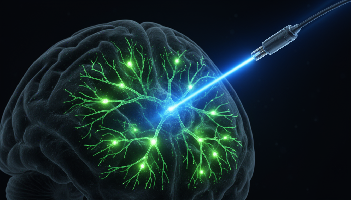
In neuroscience, we can think of techniques like optogenetics as a biological equivalent of an RCT (see Chapter 6 for detailed coverage of neurostimulation techniques). By using light to activate or deactivate specific neurons, we can observe the effect of this intervention on the activity of other neurons or on the behavior of the animal.
However, it is not always possible to perform an RCT. In many cases, we are limited to observational data, where we can only observe the system without intervening. In these cases, we must be careful to avoid the trap of assuming that “correlation implies causation”.
Judea Pearl’s Causal Hierarchy
Judea Pearl introduced a three-level hierarchy of causal reasoning:
- Association (Seeing): \(P(Y|X)\) - What is the probability of Y given that we observe X?
- Intervention (Doing): \(P(Y|do(X))\) - What is the probability of Y if we intervene to set X?
- Counterfactuals (Imagining): \(P(Y_x|X',Y')\) - What would have happened if X had been different?
The key distinction is between seeing and doing. When we observe that X and Y co-occur, we cannot conclude that setting X will cause Y. We need intervention or a causal model.
15.2 9.2 The Pitfalls of Correlation
A common mistake in scientific analysis is to assume that a correlation between two variables implies a causal relationship. While it’s true that causal relationships often produce correlations, the reverse is not guaranteed. A correlation can arise for several reasons that don’t involve a direct causal link.
The most common reason for a misleading correlation is a confounding variable. A confounder is a third, often unobserved, variable that influences both of the variables being measured. For example, imagine we observe a correlation between the firing rate of a neuron in the visual cortex and a neuron in the motor cortex. It might be tempting to conclude that the visual neuron is causing the motor neuron to fire. However, it’s more likely that both neurons are being driven by a third factor: the presentation of a visual stimulus that requires a motor response. In this case, the stimulus is the confounding variable.
Without the ability to perform an intervention (like silencing the visual neuron and observing the motor neuron’s response), it is very difficult to disentangle these kinds of spurious correlations from true causal relationships based on observational data alone.
Common Causal Structures
There are three fundamental causal structures that create correlations:
- Chain: \(A \rightarrow B \rightarrow C\) (A causes B causes C)
- Fork (Common Cause): \(A \leftarrow B \rightarrow C\) (B causes both A and C)
- Collider (Common Effect): \(A \rightarrow B \leftarrow C\) (Both A and C cause B)
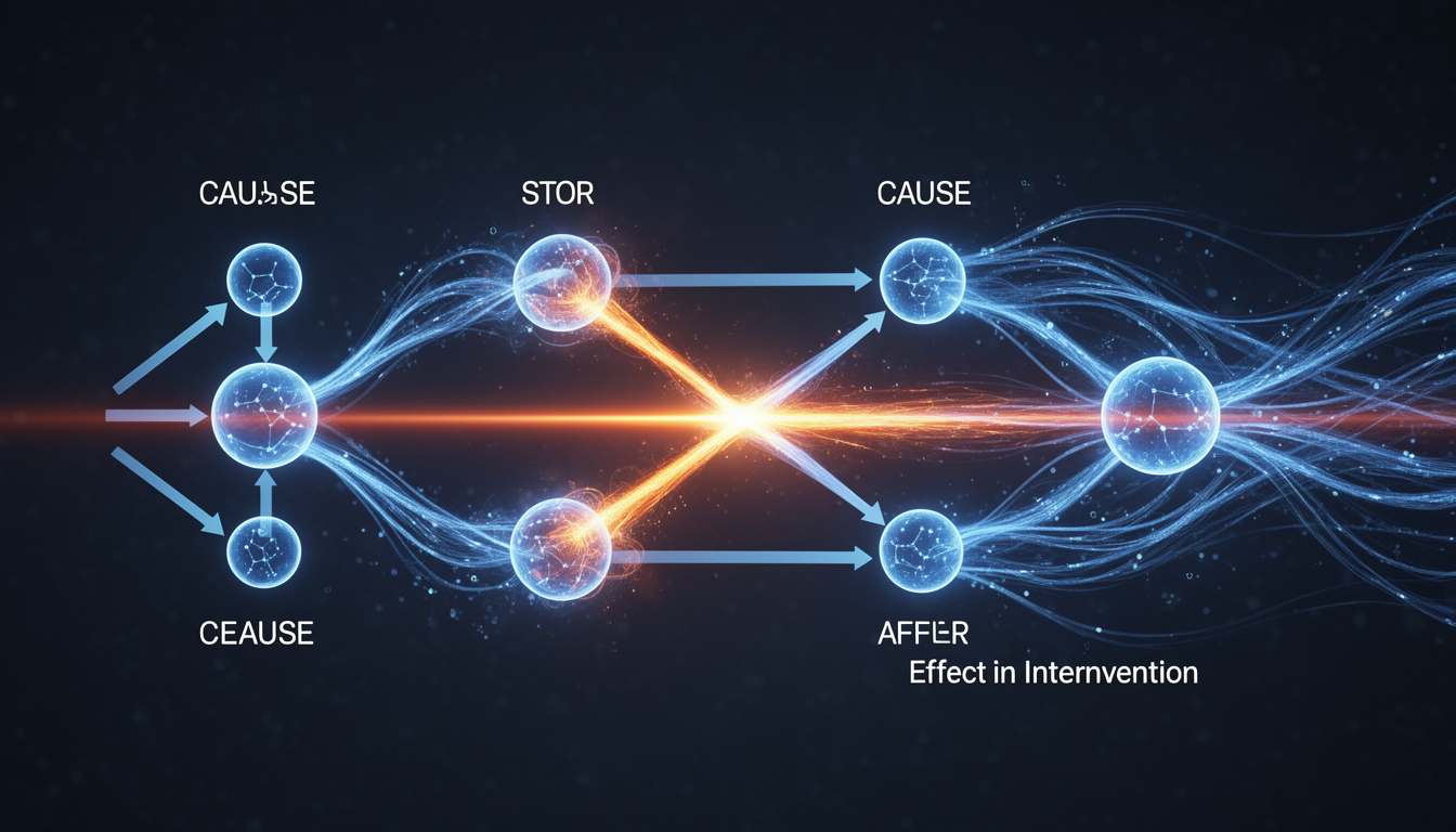
 Figure 9.1: Common causal graph structures. Left: Chain (X → Z → Y). Center: Fork/Confounder (X ← Z → Y). Right: Collider (X → Z ← Y). Conditioning on Z blocks chains and forks but opens colliders. Understanding this is crucial for causal inference.
Understanding these structures is crucial for identifying confounders and designing appropriate statistical controls.
15.3 9.3 Causal Graphs and DAGs
Directed Acyclic Graphs (DAGs) provide a formal language for representing causal relationships. In a DAG: - Nodes represent variables - Directed edges (arrows) represent direct causal effects - The graph must be acyclic (no loops)
Code Lab: Building Causal DAGs
Interpretation: In this DAG, the Stimulus is a confounder - it causes both V1 and Motor activity. If we only observe correlations between V1 and Motor, we cannot tell if: - V1 causes Motor (direct effect) - Stimulus causes both (confounding) - Both mechanisms are present
This is exactly the problem optogenetics solves: by directly manipulating V1 with light, we can measure the direct causal effect V1 → Motor.
15.4 9.4 Pearl’s Do-Calculus and Interventions
The \(do(\cdot)\) operator represents an intervention where we force a variable to take a specific value, breaking incoming causal arrows.
Key difference: - Observation: \(P(Y|X=x)\) - We passively observe X=x and measure Y - Intervention: \(P(Y|do(X=x))\) - We actively set X=x and measure Y
 Figure 9.2: The fundamental distinction between observation P(Y|X) and intervention P(Y|do(X)). Observation includes confounding paths, while intervention surgically removes incoming arrows to the treatment node, revealing the true causal effect. This is why randomized controlled trials are the gold standard.
Example: Optogenetics as an Intervention
def simulate_optogenetics_experiment(n_trials=1000):
    """
    Simulate an optogenetics experiment demonstrating causal inference.

    Scenario:
    - Stimulus → V1 activity
    - Stimulus → Motor activity
    - V1 → Motor activity (direct effect we want to measure)

    We compare:
    1. Observational: P(Motor | V1=high)
    2. Interventional: P(Motor | do(V1=high)) using optogenetics
    """
    np.random.seed(42)

    # Generate data
    stimulus_strength = np.random.randn(n_trials)

    # Observational data (natural correlations)
    v1_natural = 0.8 * stimulus_strength + np.random.randn(n_trials) * 0.3
    motor_natural = 0.5 * stimulus_strength + 0.3 * v1_natural + np.random.randn(n_trials) * 0.3

    # Interventional data (optogenetics forces V1 activity)
    v1_opto = np.random.choice([0, 2], n_trials)  # Either off or strongly activated
    motor_opto = 0.5 * stimulus_strength + 0.3 * v1_opto + np.random.randn(n_trials) * 0.3

    # Analysis
    fig, axes = plt.subplots(1, 2, figsize=(12, 5))

    # Observational correlation
    axes[0].scatter(v1_natural, motor_natural, alpha=0.3, c='#0066cc')
    axes[0].set_xlabel('V1 Activity (observed)')
    axes[0].set_ylabel('Motor Activity')
    axes[0].set_title('Observational Data - (Correlation includes confounding)')

    # Add regression line
    z = np.polyfit(v1_natural, motor_natural, 1)
    p = np.poly1d(z)
    x_line = np.linspace(v1_natural.min(), v1_natural.max(), 100)
    axes[0].plot(x_line, p(x_line), "r-", linewidth=2,
                 label=f'Slope: {z[0]:.2f}')
    axes[0].legend()

    # Interventional (optogenetics)
    for opto_level in [0, 2]:
        mask = v1_opto == opto_level
        label = 'Opto OFF' if opto_level == 0 else 'Opto ON'
        color = '#cccccc' if opto_level == 0 else '#cc0000'
        axes[1].scatter(v1_opto[mask], motor_opto[mask],
                       alpha=0.3, c=color, label=label)

    axes[1].set_xlabel('V1 Activity (manipulated)')
    axes[1].set_ylabel('Motor Activity')
    axes[1].set_title('Interventional Data (Optogenetics) - (Direct causal effect)')
    axes[1].legend()

    # Calculate causal effect
    motor_opto_on = motor_opto[v1_opto == 2].mean()
    motor_opto_off = motor_opto[v1_opto == 0].mean()
    causal_effect = motor_opto_on - motor_opto_off

    fig.suptitle(f'True Causal Effect: {0.3 * 2:.2f}, Estimated: {causal_effect:.2f}',
                 fontsize=12, y=1.02)
    plt.tight_layout()

    return fig

# simulate_optogenetics_experiment()
Key Insight: The observational correlation includes both the direct effect (V1 → Motor) and confounding (Stimulus → V1, Stimulus → Motor). The interventional approach isolates the direct causal effect.
15.5 9.5 Estimating Causal Effects from Observational Data
When direct intervention is not possible, we are not entirely lost. Several statistical methods have been developed to estimate causal effects from purely observational data. While these methods are not as foolproof as an RCT, they can provide valuable evidence for or against a causal hypothesis.
Regression with Confounding Control
One common approach is regression analysis. By fitting a statistical model that includes not only the variable of interest but also potential confounding variables, we can attempt to “control for” the influence of the confounders. The goal is to isolate the unique relationship between the variable of interest and the outcome. However, this method is only as good as our ability to identify and measure all relevant confounders. If a significant confounder is left out of the model, the results can still be biased.
def demonstrate_confounding_control():
    """
    Show how controlling for confounders in regression reveals causal effects.
    """
    np.random.seed(42)
    n = 500

    # True causal structure:
    # Confounder → Treatment
    # Confounder → Outcome
    # Treatment → Outcome (this is what we want to estimate)

    confounder = np.random.randn(n)
    treatment = 0.8 * confounder + np.random.randn(n) * 0.5
    outcome = 0.5 * treatment + 1.2 * confounder + np.random.randn(n) * 0.3

    # Naive regression (ignoring confounder)
    from sklearn.linear_model import LinearRegression

    model_naive = LinearRegression()
    model_naive.fit(treatment.reshape(-1, 1), outcome)
    effect_naive = model_naive.coef_[0]

    # Proper regression (controlling for confounder)
    X_controlled = np.column_stack([treatment, confounder])
    model_controlled = LinearRegression()
    model_controlled.fit(X_controlled, outcome)
    effect_controlled = model_controlled.coef_[0]

    print(f"True causal effect: 0.50")
    print(f"Naive estimate (no control): {effect_naive:.2f}")
    print(f"Controlled estimate: {effect_controlled:.2f}")

    return effect_naive, effect_controlled

# demonstrate_confounding_control()
Instrumental Variables
Another powerful technique is the use of instrumental variables (IV). An instrumental variable is a variable that: 1. Is correlated with the treatment/exposure (relevance) 2. Affects the outcome only through the treatment (exclusion restriction) 3. Is not correlated with unmeasured confounders (independence)
Neuroscience Example: In studying the effect of dopamine on learning, we might use a genetic variant that affects dopamine receptor density as an instrument. The genetic variant: - Affects dopamine signaling (relevance) - Affects learning only through dopamine, not through other pathways (exclusion) - Is randomly assigned at birth (independence from confounders)
def instrumental_variable_example():
    """
    Demonstrate instrumental variable estimation.
    """
    np.random.seed(42)
    n = 1000

    # True causal structure:
    # Instrument → Treatment
    # Treatment → Outcome
    # Unmeasured confounder → Treatment
    # Unmeasured confounder → Outcome

    instrument = np.random.randn(n)  # e.g., genetic variant
    unmeasured = np.random.randn(n)  # e.g., socioeconomic factors

    treatment = 0.6 * instrument + 0.5 * unmeasured + np.random.randn(n) * 0.3
    outcome = 0.8 * treatment + 0.7 * unmeasured + np.random.randn(n) * 0.3

    # Naive OLS (biased due to unmeasured confounder)
    from sklearn.linear_model import LinearRegression

    model_ols = LinearRegression()
    model_ols.fit(treatment.reshape(-1, 1), outcome)
    effect_ols = model_ols.coef_[0]

    # Two-stage least squares (IV estimation)
    # Stage 1: Regress treatment on instrument
    model_stage1 = LinearRegression()
    model_stage1.fit(instrument.reshape(-1, 1), treatment)
    treatment_predicted = model_stage1.predict(instrument.reshape(-1, 1))

    # Stage 2: Regress outcome on predicted treatment
    model_stage2 = LinearRegression()
    model_stage2.fit(treatment_predicted.reshape(-1, 1), outcome)
    effect_iv = model_stage2.coef_[0]

    print(f"True causal effect: 0.80")
    print(f"OLS estimate (biased): {effect_ols:.2f}")
    print(f"IV estimate (unbiased): {effect_iv:.2f}")

    return effect_ols, effect_iv

# instrumental_variable_example()
15.6 9.6 Causal Discovery from Data
Can we learn causal structure from observational data alone? Under certain assumptions, yes. Causal discovery algorithms search over possible DAGs to find structures consistent with the observed data.
PC Algorithm
The PC algorithm (named after Peter Spirtes and Clark Glymour) uses conditional independence tests to infer causal structure.
def demonstrate_pc_algorithm():
    """
    Demonstrate causal discovery using the PC algorithm.

    Note: This is a simplified illustration. Real applications should use
    dedicated libraries like causal-learn or py-causal.
    """
    import networkx as nx
    from scipy.stats import pearsonr

    np.random.seed(42)
    n = 1000

    # Generate data from known causal structure
    # True structure: X → Y → Z, X → Z
    X = np.random.randn(n)
    Y = 0.7 * X + np.random.randn(n) * 0.3
    Z = 0.5 * Y + 0.4 * X + np.random.randn(n) * 0.3

    data = np.column_stack([X, Y, Z])
    var_names = ['X', 'Y', 'Z']

    # Step 1: Start with fully connected graph
    G = nx.DiGraph()
    G.add_nodes_from(var_names)
    for i in range(len(var_names)):
        for j in range(len(var_names)):
            if i != j:
                G.add_edge(var_names[i], var_names[j])

    # Step 2: Remove edges based on conditional independence
    # (Simplified version - real PC algorithm is more sophisticated)

    # Check if X and Z are independent given Y
    from sklearn.linear_model import LinearRegression

    def partial_correlation(x, y, z):
        """Compute partial correlation of x and y given z."""
        model_xz = LinearRegression().fit(z.reshape(-1, 1), x)
        residual_x = x - model_xz.predict(z.reshape(-1, 1))

        model_yz = LinearRegression().fit(z.reshape(-1, 1), y)
        residual_y = y - model_yz.predict(z.reshape(-1, 1))

        corr, p_value = pearsonr(residual_x, residual_y)
        return corr, p_value

    # Test: Are X and Z independent given Y?
    corr_xz_given_y, p_value = partial_correlation(X, Z, Y)
    print(f"Partial correlation X-Z | Y: {corr_xz_given_y:.3f} (p={p_value:.3f})")
    print(f"X and Z are {'independent' if p_value > 0.05 else 'dependent'} given Y")
    print("Therefore, there must be a direct edge X → Z in the true graph")

    return G

# demonstrate_pc_algorithm()
15.7 9.7 Causal Inference in AI
The principles of causal inference are becoming increasingly important in the field of AI, particularly in the subfield of explainable AI (XAI). As AI models become more complex and are deployed in high-stakes domains like medicine and finance, it is no longer enough for them to simply make accurate predictions. We also need to understand why they are making those predictions.
Network Ablation as Intervention
In deep learning, we can perform interventional experiments analogous to optogenetics:
def neural_network_ablation_example():
    """
    Demonstrate causal inference in neural networks through ablation.

    Question: Does a particular layer/neuron cause the network's prediction?
    Method: Ablate (set to zero) and measure effect on output.
    """
    import torch
    import torch.nn as nn

    # Simple neural network
    model = nn.Sequential(
        nn.Linear(10, 20),
        nn.ReLU(),
        nn.Linear(20, 10),
        nn.ReLU(),
        nn.Linear(10, 2)
    )

    # Generate random input
    x = torch.randn(1, 10)

    # Normal forward pass
    output_normal = model(x)
    pred_normal = torch.argmax(output_normal, dim=1).item()

    # Ablate second layer (set to zero)
    def forward_with_ablation(model, x, layer_idx):
        """Forward pass with specified layer ablated."""
        with torch.no_grad():
            out = x
            for i, layer in enumerate(model):
                out = layer(out)
                if i == layer_idx:
                    out = torch.zeros_like(out)  # Ablation
            return out

    output_ablated = forward_with_ablation(model, x, layer_idx=2)
    pred_ablated = torch.argmax(output_ablated, dim=1).item()

    print(f"Normal prediction: class {pred_normal}")
    print(f"Ablated prediction: class {pred_ablated}")
    print(f"Causal effect of layer 2: {'None' if pred_normal == pred_ablated else 'Significant'}")

    return pred_normal, pred_ablated

# neural_network_ablation_example()
Causal Models for Robust AI
Causal models can provide a framework for understanding the internal workings of a “black box” AI model. By treating the model’s internal components (like artificial neurons) as variables in a causal system, we can use interventional and observational techniques to map out the causal relationships between them. This can help us to identify the key features that are driving the model’s decisions and to ensure that the model is not relying on spurious correlations in the training data.
Furthermore, a causal understanding of AI models can help us to make them more robust and reliable. If we understand the causal mechanisms that underlie a model’s behavior, we can better predict how it will behave in new, unseen situations and we can design interventions to correct for undesirable behavior.
15.8 Exercises
Conceptual Questions
Correlation vs. Causation: Explain why observing that variable X and Y are correlated does not imply that X causes Y. Provide a neuroscience example where correlation does not equal causation.
DAG Interpretation: Draw a DAG for the following scenario: “Dopamine levels affect both motivation and learning performance, and motivation also affects learning performance.” Identify which correlations can and cannot be attributed to direct causal effects.
Confounding: In a study, researchers observe that people who drink more coffee have better memory. Before concluding that coffee improves memory, what potential confounders should they consider?
Computational Problems
Build a Causal DAG: Create a causal DAG for a visual decision-making task with the following variables: Visual Stimulus, V1 Activity, V4 Activity, Prefrontal Activity, Motor Response, and Reward. Use Python and NetworkX to visualize your DAG.
Simulate Confounding: Generate synthetic data where a confounder Z causes both treatment X and outcome Y. Show that:
- Regressing Y on X alone gives a biased estimate
- Regressing Y on both X and Z gives an unbiased estimate of X’s causal effect
Instrumental Variable: Implement two-stage least squares regression to estimate a causal effect using an instrumental variable. Compare your IV estimate to the naive OLS estimate.
Discussion Questions
Optogenetics vs. Correlation: Why is optogenetics considered the “gold standard” for establishing causality in neuroscience? What are its limitations?
AI Interpretability: How can causal reasoning improve AI interpretability and robustness? Provide an example where understanding causal mechanisms would prevent an AI system from making errors.
Ethics of Causation: In healthcare AI, why is it important to distinguish between causal and correlational relationships when making treatment recommendations? What could go wrong if an AI system only learns correlations?
15.9 References
Pearl, J., & Mackenzie, D. (2018). The Book of Why: The New Science of Cause and Effect. Basic Books.
Pearl, J. (2009). Causality: Models, Reasoning, and Inference (2nd ed.). Cambridge University Press.
Spirtes, P., Glymour, C., & Scheines, R. (2000). Causation, Prediction, and Search (2nd ed.). MIT Press.
Peters, J., Janzing, D., & Schölkopf, B. (2017). Elements of Causal Inference: Foundations and Learning Algorithms. MIT Press.
Hernán, M. A., & Robins, J. M. (2020). Causal Inference: What If. Chapman & Hall/CRC.
Angrist, J. D., & Pischke, J. S. (2008). Mostly Harmless Econometrics: An Empiricist’s Companion. Princeton University Press.
Deisseroth, K. (2015). Optogenetics: 10 years of microbial opsins in neuroscience. Nature Neuroscience, 18(9), 1213-1225.
Schölkopf, B., Locatello, F., Bauer, S., et al. (2021). Toward Causal Representation Learning. Proceedings of the IEEE, 109(5), 612-634.
Glymour, C., Zhang, K., & Spirtes, P. (2019). Review of Causal Discovery Methods Based on Graphical Models. Frontiers in Genetics, 10, 524.