20  Deep Learning: Training & Optimisation

NoteLearning Objectives

By the end of this chapter, you will be able to:

• Master deep neural network architectures and training techniques
• Understand optimization algorithms and their underlying mathematical principles
• Implement key deep learning components from scratch and with frameworks
• Apply best practices for model development and troubleshooting
• Compare biological and artificial optimization approaches

20.1 13.1 Neural Network Fundamentals

Figure 20.1: Deep neural networks transform data through successive layers of abstraction, from raw inputs to high-level representations.

Deep learning has revolutionized AI by enabling models to learn hierarchical representations directly from data. At its core, deep learning is built on neural networks with multiple layers that progressively extract higher-level features.

Figure 13.1: A multilayer perceptron with two hidden layers, showing how neurons connect between layers and activate through non-linear functions.

13.1.1 Multilayer Perceptrons

Multilayer perceptrons (MLPs) are the foundational architecture of deep learning, consisting of an input layer, one or more hidden layers, and an output layer.

import numpy as np
import matplotlib.pyplot as plt
import torch
import torch.nn as nn
import torch.optim as optim

    # Define a simple MLP using PyTorch
class SimpleMLP(nn.Module):
    def __init__(self, input_size, hidden_sizes, output_size):
        """
        A basic multilayer perceptron implementation.
        
        Args:
            input_size: Number of input features
            hidden_sizes: List of hidden layer sizes
            output_size: Number of output units
        """
        super(SimpleMLP, self).__init__()
        
        # Create a list to hold all layers
        layers = []
        
        # Input layer to first hidden layer
        layers.append(nn.Linear(input_size, hidden_sizes[0]))
        layers.append(nn.ReLU())
        
        # Hidden layers
        for i in range(len(hidden_sizes) - 1):
            layers.append(nn.Linear(hidden_sizes[i], hidden_sizes[i+1]))
            layers.append(nn.ReLU())
        
        # Final layer
        layers.append(nn.Linear(hidden_sizes[-1], output_size))
        
        # Combine all layers into a sequential model
        self.model = nn.Sequential(*layers)
    
    def forward(self, x):
        """Forward pass through the network."""
        return self.model(x)

    # Create an example MLP
input_size = 10
hidden_sizes = [128, 64, 32]
output_size = 2
model = SimpleMLP(input_size, hidden_sizes, output_size)

    # Display model architecture
print(model)

The power of MLPs comes from their ability to approximate any continuous function with sufficient neurons in the hidden layers (universal approximation theorem).

Figure 20.2: Backpropagation - error signals flowing backward through network layers like reverse waterfalls of light, gradient information cascading from output to input.

13.1.2 Activation Functions

Activation functions introduce non-linearity into neural networks, allowing them to learn complex patterns.

def plot_activation_functions():
    """Plot common activation functions used in deep learning."""
    # Generate input values
    x = np.linspace(-5, 5, 1000)
    
    # Calculate activation function outputs
    sigmoid = 1 / (1 + np.exp(-x))
    tanh = np.tanh(x)
    relu = np.maximum(0, x)
    leaky_relu = np.where(x > 0, x, 0.1 * x)
    elu = np.where(x > 0, x, np.exp(x) - 1)
    
    # Create plot
    plt.figure(figsize=(12, 8))
    
    plt.plot(x, sigmoid, label='Sigmoid')
    plt.plot(x, tanh, label='Tanh')
    plt.plot(x, relu, label='ReLU')
    plt.plot(x, leaky_relu, label='Leaky ReLU')
    plt.plot(x, elu, label='ELU')
    
    plt.grid(True)
    plt.legend()
    plt.title('Common Activation Functions')
    plt.xlabel('Input')
    plt.ylabel('Output')
    plt.axhline(y=0, color='k', linestyle='-', alpha=0.3)
    plt.axvline(x=0, color='k', linestyle='-', alpha=0.3)
    
    plt.tight_layout()
    return plt

Common activation functions include:

• ReLU (Rectified Linear Unit): \(f(x) = \max(0, x)\)
  • Pros: Fast computation, reduces vanishing gradient problem
  • Cons: “Dying ReLU” problem (neurons can get stuck)
• Leaky ReLU: \(f(x) = \max(\alpha x, x)\) where \(\alpha\) is a small constant
  • Pros: Addresses dying ReLU problem
  • Cons: Performance improvement is often marginal
• Sigmoid: \(f(x) = \frac{1}{1 + e^{-x}}\)
  • Pros: Outputs between 0 and 1, useful for binary classification
  • Cons: Vanishing gradient problem for extreme inputs
• Tanh (Hyperbolic Tangent): \(f(x) = \tanh(x) = \frac{e^x - e^{-x}}{e^x + e^{-x}}\)
  • Pros: Zero-centered, useful in recurrent networks
  • Cons: Still suffers from vanishing gradient
• GELU (Gaussian Error Linear Unit): \(f(x) = x \cdot \Phi(x)\) where \(\Phi\) is the CDF of the standard normal distribution
  • Pros: Smooth, better performance in transformers
  • Cons: More computationally expensive

Recent architectures like transformers commonly use GELU, while CNNs often use ReLU or its variants.

13.1.3 Backpropagation Algorithm

Backpropagation is the cornerstone algorithm for training neural networks, efficiently computing gradients through the chain rule.

def manual_backpropagation_example():
    """
    Demonstrate backpropagation with a simple 2-layer network.
    """
    # Simple network: Input -> Hidden (2 neurons) -> Output
    # Forward pass
    def sigmoid(x):
        return 1 / (1 + np.exp(-x))
    
    def sigmoid_derivative(x):
        return x * (1 - x)
    
    # Network parameters
    input_size = 3
    hidden_size = 2
    output_size = 1
    
    # Inputs and target
    X = np.array([[0.1, 0.2, 0.3]])
    y_true = np.array([[0.7]])
    
    # Initialize weights and biases
    np.random.seed(42)
    W1 = np.random.randn(input_size, hidden_size)
    b1 = np.zeros((1, hidden_size))
    W2 = np.random.randn(hidden_size, output_size)
    b2 = np.zeros((1, output_size))
    
    # Forward pass
    hidden_input = np.dot(X, W1) + b1
    hidden_output = sigmoid(hidden_input)
    final_input = np.dot(hidden_output, W2) + b2
    y_pred = sigmoid(final_input)
    
    # Calculate loss
    loss = 0.5 * np.sum((y_pred - y_true) ** 2)
    
    # Backpropagation
    # Output layer error
    output_error = y_pred - y_true
    output_delta = output_error * sigmoid_derivative(y_pred)
    
    # Hidden layer error
    hidden_error = np.dot(output_delta, W2.T)
    hidden_delta = hidden_error * sigmoid_derivative(hidden_output)
    
    # Update weights and biases
    learning_rate = 0.1
    W2 -= learning_rate * np.dot(hidden_output.T, output_delta)
    b2 -= learning_rate * np.sum(output_delta, axis=0, keepdims=True)
    W1 -= learning_rate * np.dot(X.T, hidden_delta)
    b1 -= learning_rate * np.sum(hidden_delta, axis=0, keepdims=True)
    
    return {
        'Initial prediction': y_pred[0][0],
        'Target': y_true[0][0],
        'Loss': loss,
        'Output delta': output_delta[0][0],
        'Hidden delta': hidden_delta[0]
    }

The backpropagation algorithm:

1. Forward Pass: Compute outputs of all neurons from input to output
2. Error Calculation: Compare network output with target to compute error
3. Backward Pass: Propagate error backward to assign “responsibility” to each parameter
4. Parameter Update: Adjust weights and biases using calculated gradients

While modern deep learning frameworks handle these calculations automatically through automatic differentiation, understanding backpropagation is crucial for developing intuition about neural network training.

13.1.4 Vanishing/Exploding Gradients

As neural networks get deeper, the problem of vanishing or exploding gradients becomes more severe:

def demonstrate_gradient_problems():
    """
    Visualize vanishing/exploding gradient problems in deep networks.
    """
    depths = list(range(1, 21))
    
    # Vanishing gradient with sigmoid
    vanishing_grads = [0.25 ** d for d in depths]
    
    # Exploding gradient with poor initialization
    exploding_grads = [1.5 ** d for d in depths]
    
    # Plot
    plt.figure(figsize=(10, 6))
    plt.semilogy(depths, vanishing_grads, 'b-', label='Vanishing Gradient (sigmoid)')
    plt.semilogy(depths, exploding_grads, 'r-', label='Exploding Gradient (poor init)')
    plt.semilogy(depths, [0.1] * len(depths), 'g--', label='Stable Gradient (with techniques)')
    
    plt.xlabel('Network Depth (layers)')
    plt.ylabel('Gradient Magnitude (log scale)')
    plt.title('Vanishing and Exploding Gradients in Deep Networks')
    plt.legend()
    plt.grid(True)
    
    plt.tight_layout()
    return plt

Solutions to these gradient problems include:

• Careful weight initialization (e.g., He, Xavier/Glorot)
• Batch normalization
• Residual connections
• Gradient clipping
• Using activation functions that don’t saturate (e.g., ReLU)

20.2 13.2 Optimization Techniques

Training deep neural networks requires effective optimization algorithms. The choice of optimizer significantly impacts training speed and model performance.

Figure 20.3: 3D loss landscape showing mountainous terrain with valleys and saddle points, with an optimization path descending toward the global minimum.

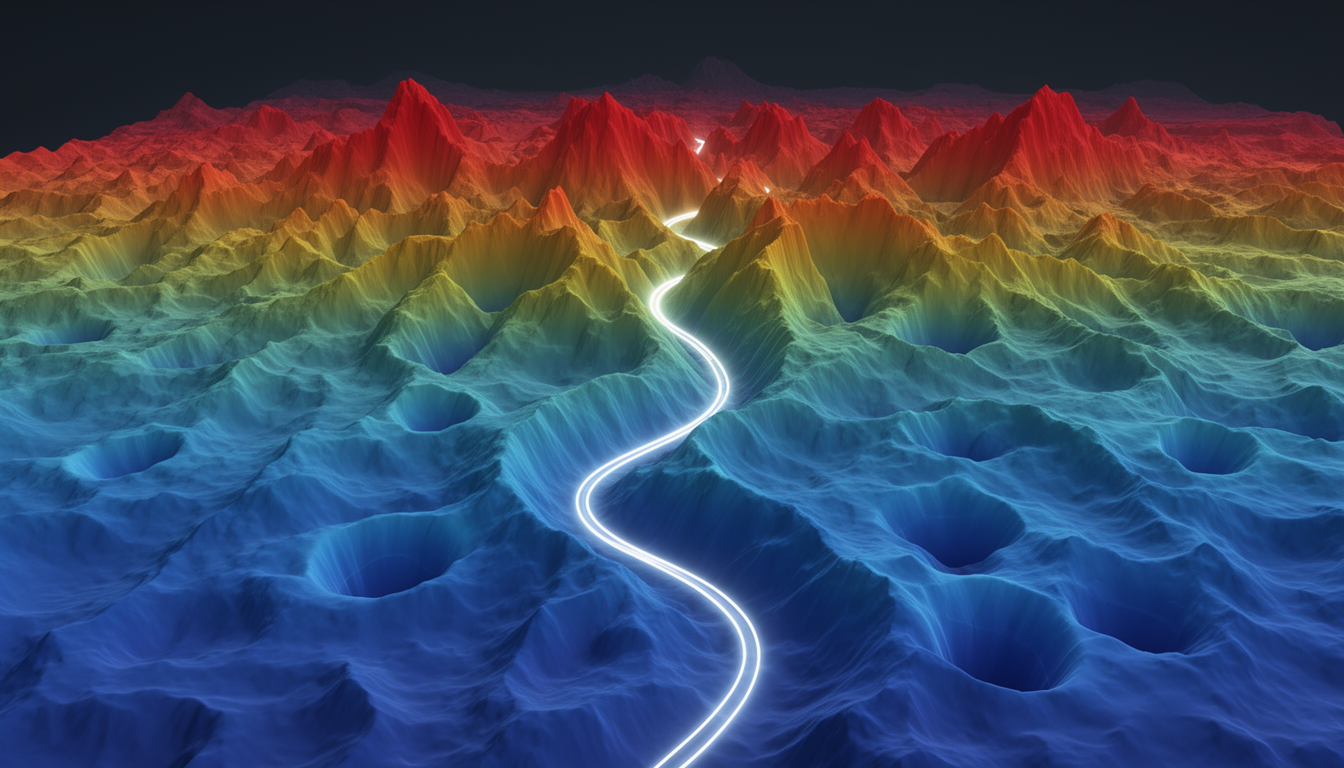
Figure 13.2: Comparison of different optimization algorithms showing convergence paths in a loss landscape. Modern approaches like Adam and RMSprop often converge faster and more reliably than vanilla SGD.

13.2.1 Stochastic Gradient Descent

Stochastic Gradient Descent (SGD) is the most fundamental optimization algorithm for neural networks:

def sgd_optimizer_example():
    """Implement basic SGD and variants."""
    # Generate dummy data
    np.random.seed(42)
    X = np.random.randn(1000, 10)
    w_true = np.random.randn(10, 1)
    y = X @ w_true + 0.1 * np.random.randn(1000, 1)
    
    # Initialize parameters
    w = np.zeros((10, 1))
    
    # SGD parameters
    learning_rate = 0.01
    batch_size = 32
    epochs = 100
    
    # Training loop
    losses = []
    for epoch in range(epochs):
        # Shuffle data
        indices = np.random.permutation(len(X))
        X_shuffled = X[indices]
        y_shuffled = y[indices]
        
        epoch_losses = []
        # Process mini-batches
        for i in range(0, len(X), batch_size):
            X_batch = X_shuffled[i:i+batch_size]
            y_batch = y_shuffled[i:i+batch_size]
            
            # Forward pass
            y_pred = X_batch @ w
            loss = np.mean((y_pred - y_batch) ** 2)
            epoch_losses.append(loss)
            
            # Backward pass (compute gradient)
            grad = 2 * X_batch.T @ (y_pred - y_batch) / batch_size
            
            # Update parameters
            w = w - learning_rate * grad
        
        losses.append(np.mean(epoch_losses))
    
    return {
        'weights': w,
        'true_weights': w_true,
        'final_loss': losses[-1],
        'loss_history': losses
    }

SGD variants include: - Batch Gradient Descent: Uses the entire dataset per update - Mini-batch SGD: Uses small batches (typically 32-256 samples) - Online SGD: Updates using one sample at a time

13.2.2 Momentum and Adaptive Methods

Modern optimizers build upon SGD by introducing momentum or adaptive learning rates:

def compare_optimizers():
    """Compare convergence speed of different optimizers."""
    import torch
    import torch.nn as nn
    import torch.optim as optim
    
    # Define a simple problem
    X = torch.randn(1000, 20)
    y = torch.randn(1000, 1)
    
    # Define model
    model = nn.Sequential(
        nn.Linear(20, 64),
        nn.ReLU(),
        nn.Linear(64, 1)
    )
    
    # Loss function
    criterion = nn.MSELoss()
    
    # Define optimizers
    optimizers = {
        'SGD': optim.SGD(model.parameters(), lr=0.01),
        'SGD+Momentum': optim.SGD(model.parameters(), lr=0.01, momentum=0.9),
        'Adam': optim.Adam(model.parameters(), lr=0.01),
        'RMSprop': optim.RMSprop(model.parameters(), lr=0.01),
        'AdamW': optim.AdamW(model.parameters(), lr=0.01, weight_decay=1e-4)
    }
    
    # Training loops
    results = {}
    
    for name, optimizer in optimizers.items():
        # Reset model
        model = nn.Sequential(
            nn.Linear(20, 64),
            nn.ReLU(),
            nn.Linear(64, 1)
        )
        
        # Train
        losses = []
        for epoch in range(100):
            optimizer.zero_grad()
            outputs = model(X)
            loss = criterion(outputs, y)
            losses.append(loss.item())
            loss.backward()
            optimizer.step()
        
        results[name] = losses
    
    # Plot
    plt.figure(figsize=(10, 6))
    for name, loss_history in results.items():
        plt.plot(loss_history, label=name)
    
    plt.xlabel('Epoch')
    plt.ylabel('Loss')
    plt.title('Optimizer Convergence Comparison')
    plt.legend()
    plt.yscale('log')
    plt.grid(True)
    
    plt.tight_layout()
    return plt

Key optimization algorithms include:

• SGD with Momentum: Adds a fraction of the previous update to the current one, helping to escape local minima and accelerate convergence
  • \(v_t = \gamma v_{t-1} + \eta - abla_\theta J(\theta)\)
  • \(\theta = \theta - v_t\)
• Nesterov Accelerated Gradient: Computes gradient at the “looked-ahead” position for better convergence
  • \(v_t = \gamma v_{t-1} + \eta - abla_\theta J(\theta - \gamma v_{t-1})\)
  • \(\theta = \theta - v_t\)
• AdaGrad: Adapts learning rates per-parameter based on historical gradients
  • \(\theta_{t+1} = \theta_t - \frac{\eta}{\sqrt{G_t + \epsilon}} \odot g_t\)
• RMSprop: Modifies AdaGrad to better handle non-convex functions by using an exponentially weighted moving average
  • \(E[g^2]_t = \beta E[g^2]_{t-1} + (1-\beta) g_t^2\)
  • \(\theta_{t+1} = \theta_t - \frac{\eta}{\sqrt{E[g^2]_t + \epsilon}} g_t\)
• Adam: Combines momentum and RMSprop ideas for robust performance
  • \(m_t = \beta_1 m_{t-1} + (1-\beta_1) g_t\) (momentum)
  • \(v_t = \beta_2 v_{t-1} + (1-\beta_2) g_t^2\) (RMSprop)
  • \(\hat{m}_t = \frac{m_t}{1-\beta_1^t}\), \(\hat{v}_t = \frac{v_t}{1-\beta_2^t}\) (bias correction)
  • \(\theta_{t+1} = \theta_t - \frac{\eta}{\sqrt{\hat{v}_t} + \epsilon} \hat{m}_t\)

Adam is currently the most widely used optimizer due to its robustness across different architectures and datasets.

13.2.3 Learning Rate Schedules

Learning rate scheduling can significantly improve training outcomes:

def learning_rate_schedules():
    """Visualize common learning rate schedules."""
    epochs = np.arange(1, 101)
    
    # Constant
    constant_lr = [0.1] * 100
    
    # Step decay
    step_lr = [0.1 * (0.1 ** (e // 30)) for e in epochs]
    
    # Exponential decay
    exp_lr = [0.1 * np.exp(-0.03 * e) for e in epochs]
    
    # Cosine annealing
    cosine_lr = [0.1 * (1 + np.cos(np.pi * e / 100)) / 2 for e in epochs]
    
    # Linear warmup + cosine decay
    warmup = 10
    warmup_cosine_lr = []
    for e in epochs:
        if e <= warmup:
            lr = 0.1 * e / warmup
        else:
            lr = 0.1 * (1 + np.cos(np.pi * (e - warmup) / (100 - warmup))) / 2
        warmup_cosine_lr.append(lr)
    
    # Plot
    plt.figure(figsize=(10, 6))
    plt.plot(epochs, constant_lr, label='Constant')
    plt.plot(epochs, step_lr, label='Step Decay')
    plt.plot(epochs, exp_lr, label='Exponential Decay')
    plt.plot(epochs, cosine_lr, label='Cosine Annealing')
    plt.plot(epochs, warmup_cosine_lr, label='Warmup + Cosine')
    
    plt.xlabel('Epoch')
    plt.ylabel('Learning Rate')
    plt.title('Learning Rate Schedules')
    plt.legend()
    plt.yscale('log')
    plt.grid(True)
    
    plt.tight_layout()
    return plt

Popular learning rate schedules include:

• Step Decay: Reduces learning rate by a factor after a set number of epochs
• Exponential Decay: Continuously decreases learning rate using an exponential function
• Cosine Annealing: Smoothly decreases learning rate following a cosine curve
• Cyclic Learning Rates: Cycles between lower and upper learning rate bounds
• One-Cycle Policy: Increases learning rate to a maximum, then decreases it
• Warmup + Decay: Gradually increases learning rate during initial epochs, then decays

13.2.4 Second-order Methods

While first-order methods like SGD use only gradient information, second-order methods incorporate curvature information:

def second_order_methods():
    """Compare first and second-order optimization methods."""
    # Generate a 2D quadratic function with conditioning issues
    def f(x, y):
        return 0.01 * x**2 + 5 * y**2
    
    def grad_f(x, y):
        return np.array([0.02 * x, 10 * y])
    
    def hessian_f(x, y):
        return np.array([[0.02, 0], [0, 10]])
    
    # Starting point
    x0, y0 = 10.0, 2.0
    
    # SGD trajectory
    sgd_path = [(x0, y0)]
    x, y = x0, y0
    lr = 0.1
    for _ in range(20):
        g = grad_f(x, y)
        x -= lr * g[0]
        y -= lr * g[1]
        sgd_path.append((x, y))
    
    # Newton's method trajectory
    newton_path = [(x0, y0)]
    x, y = x0, y0
    for _ in range(5):  # Usually converges in fewer steps
        g = grad_f(x, y)
        H = hessian_f(x, y)
        H_inv = np.linalg.inv(H)
        update = H_inv @ g
        x -= update[0]
        y -= update[1]
        newton_path.append((x, y))
    
    # Plot
    x_range = np.linspace(-10, 10, 100)
    y_range = np.linspace(-2, 2, 100)
    X, Y = np.meshgrid(x_range, y_range)
    Z = f(X, Y)
    
    plt.figure(figsize=(10, 8))
    
    # Contour plot
    plt.contour(X, Y, Z, 20, cmap='viridis', alpha=0.6)
    
    # Plot paths
    sgd_path = np.array(sgd_path)
    newton_path = np.array(newton_path)
    
    plt.plot(sgd_path[:, 0], sgd_path[:, 1], 'r.-', label='SGD', linewidth=2, markersize=8)
    plt.plot(newton_path[:, 0], newton_path[:, 1], 'b.-', label="Newton's Method", linewidth=2, markersize=8)
    
    plt.xlabel('x')
    plt.ylabel('y')
    plt.title("Comparison of First-Order vs. Second-Order Methods")
    plt.legend()
    plt.grid(True)
    
    plt.tight_layout()
    return plt

Second-order methods include:

• Newton’s Method: Uses the Hessian matrix (second derivatives) for updates
  • \(\theta_{t+1} = \theta_t - H^{-1}(\theta_t) - abla_\theta J(\theta_t)\)
  • Pros: Fast convergence near optimum
  • Cons: Expensive Hessian computation and inversion
• Quasi-Newton Methods (e.g., BFGS, L-BFGS): Approximate the Hessian
  • Pros: Faster than Newton’s method
  • Cons: Still too expensive for large neural networks
• Natural Gradient Descent: Uses the Fisher information matrix
  • Pros: Invariant to reparameterization
  • Cons: Computation and storage requirements

While second-order methods offer theoretical advantages, their computational requirements generally make them impractical for deep learning. However, approximations like K-FAC (Kronecker-Factored Approximate Curvature) are being explored to make second-order information more accessible.

20.3 13.3 Regularization Strategies

Regularization helps prevent overfitting by constraining the model’s capacity or adding noise to the training process.

Figure 13.3: Common regularization methods in deep learning, including dropout, weight decay (L2), batch normalization, data augmentation, early stopping, and label smoothing.

13.3.1 Dropout and Batch Normalization

def dropout_example():
    """Implement and visualize dropout."""
    import torch
    import torch.nn as nn
    
    # Define a model with dropout
    class MLPWithDropout(nn.Module):
        def __init__(self, dropout_rate=0.5):
            super().__init__()
            self.fc1 = nn.Linear(784, 256)
            self.dropout1 = nn.Dropout(dropout_rate)
            self.fc2 = nn.Linear(256, 128)
            self.dropout2 = nn.Dropout(dropout_rate)
            self.fc3 = nn.Linear(128, 10)
        
        def forward(self, x):
            x = torch.relu(self.fc1(x))
            x = self.dropout1(x)
            x = torch.relu(self.fc2(x))
            x = self.dropout2(x)
            x = self.fc3(x)
            return x
    
    # Create a toy example for visualization
    model = MLPWithDropout(dropout_rate=0.5)
    
    # Generate random activations for demonstration
    activations = torch.rand(1, 256)
    
    # Apply dropout with different rates
    dropout_rates = [0.0, 0.3, 0.5, 0.7]
    results = []
    
    for rate in dropout_rates:
        dropout = nn.Dropout(rate)
        # Set model to training mode
        dropout.train()
        # Apply dropout
        dropped_activations = dropout(activations)
        results.append((rate, dropped_activations[0].detach().numpy()))
    
    # Visualize
    fig, axes = plt.subplots(len(dropout_rates), 1, figsize=(10, 8))
    
    for i, (rate, acts) in enumerate(results):
        axes[i].bar(range(50), acts[:50], alpha=0.7)  # Show first 50 units
        axes[i].set_title(f'Dropout Rate: {rate}')
        axes[i].set_ylim(0, 1.5)  # Account for scaling during training
        axes[i].grid(True, alpha=0.3)
    
    plt.tight_layout()
    return fig

def batch_norm_example():
    """Demonstrate batch normalization effect."""
    import torch
    import torch.nn as nn
    
    # Create random activations
    np.random.seed(42)
    # Poorly scaled/shifted activations
    activations = np.random.randn(100, 32) * 10 + 5
    
    # Apply batch normalization
    bn = nn.BatchNorm1d(32)
    normalized = bn(torch.tensor(activations, dtype=torch.float32))
    normalized = normalized.detach().numpy()
    
    # Visualize
    fig, axes = plt.subplots(2, 1, figsize=(10, 8))
    
    # Plot raw activation distribution
    for i in range(5):  # Show first 5 features
        axes[0].hist(activations[:, i], alpha=0.3, bins=20, label=f'Feature {i+1}')
    axes[0].set_title('Before Batch Normalization')
    axes[0].grid(True, alpha=0.3)
    axes[0].legend()
    
    # Plot normalized activation distribution
    for i in range(5):
        axes[1].hist(normalized[:, i], alpha=0.3, bins=20, label=f'Feature {i+1}')
    axes[1].set_title('After Batch Normalization')
    axes[1].grid(True, alpha=0.3)
    axes[1].legend()
    
    plt.tight_layout()
    return fig

Dropout stochastically zeroes activations during training, forcing the network to learn redundant representations:

1. During training: Each neuron is kept with probability p (typically 0.5 to 0.8)
2. During inference: All neurons are used, but outputs are scaled by p

Batch Normalization normalizes activations within a mini-batch, making training more stable:

1. Normalize: \(\hat{x}_i = \frac{x_i - \mu_B}{\sqrt{\sigma_B^2 + \epsilon}}\)
2. Scale and shift: \(y_i = \gamma \hat{x}_i + \beta\)

Benefits include: - Reduced internal covariate shift - Improved gradient flow - Regularization effect - Reduced sensitivity to initialization

13.3.2 Weight Decay and Early Stopping

def weight_decay_visualization():
    """Visualize the effect of weight decay on model complexity."""
    from sklearn.linear_model import Ridge
    
    # Generate synthetic data
    np.random.seed(42)
    X = np.sort(np.random.rand(100, 1) * 6 - 3, axis=0)
    y = np.sin(X.ravel()) + np.random.normal(0, 0.1, X.shape[0])
    
    # Fit with different regularization strengths
    alphas = [0, 0.001, 0.01, 0.1, 1.0]
    degrees = 10  # polynomial degree
    
    X_plot = np.linspace(-3, 3, 1000).reshape(-1, 1)
    
    plt.figure(figsize=(12, 8))
    
    for i, alpha in enumerate(alphas):
        # Create polynomial features
        from sklearn.preprocessing import PolynomialFeatures
        from sklearn.pipeline import make_pipeline
        
        model = make_pipeline(
            PolynomialFeatures(degrees),
            Ridge(alpha=alpha)
        )
        
        model.fit(X, y)
        y_plot = model.predict(X_plot)
        
        plt.subplot(len(alphas), 1, i+1)
        plt.scatter(X, y, color='navy', s=30, marker='o', label="Training data")
        plt.plot(X_plot, y_plot, color='red', label="Model")
        plt.plot(X_plot, np.sin(X_plot.ravel()), color='green', label="True function")
        plt.title(f"Weight Decay (L2): α = {alpha}")
        plt.ylim((-1.5, 1.5))
        plt.legend()
    
    plt.tight_layout()
    return plt

def plot_early_stopping():
    """Visualize early stopping based on validation performance."""
    # Simulate training and validation losses
    epochs = np.arange(1, 101)
    
    # Training loss (continues to decrease)
    train_loss = 1.0 / (0.1 * epochs + 1.0) + 0.1
    
    # Validation loss (starts increasing after a while)
    val_loss = 1.0 / (0.1 * epochs + 1.0) + 0.1 + 0.05 * np.maximum(0, epochs - 40) / 60
    
    # Add noise
    np.random.seed(42)
    train_loss += np.random.normal(0, 0.02, len(epochs))
    val_loss += np.random.normal(0, 0.03, len(epochs))
    
    # Determine early stopping point
    patience = 10
    best_val_loss = float('inf')
    best_epoch = 0
    stop_epoch = 0
    
    for i, loss in enumerate(val_loss):
        if loss < best_val_loss:
            best_val_loss = loss
            best_epoch = i
        elif i > best_epoch + patience:
            stop_epoch = i
            break
    
    # Plot
    plt.figure(figsize=(10, 6))
    plt.plot(epochs, train_loss, 'b-', label='Training Loss')
    plt.plot(epochs, val_loss, 'r-', label='Validation Loss')
    
    # Mark early stopping point
    if stop_epoch > 0:
        plt.axvline(x=stop_epoch, color='g', linestyle='--', label=f'Early Stopping (Epoch {stop_epoch})')
    
    # Mark best validation point
    plt.axvline(x=best_epoch, color='m', linestyle=':', label=f'Best Validation (Epoch {best_epoch})')
    
    plt.xlabel('Epochs')
    plt.ylabel('Loss')
    plt.title('Early Stopping Based on Validation Loss')
    plt.legend()
    plt.grid(True)
    
    plt.tight_layout()
    return plt

Weight Decay (L2 regularization) adds a penalty term to the loss function proportional to the squared weights:

\(L_{reg} = L_{original} + \lambda \sum_i w_i^2\)

This encourages the model to use smaller weights, reducing model complexity and preventing overfitting.

Early Stopping halts training when performance on a validation set stops improving:

1. Monitor validation performance at regular intervals
2. Save the model when it achieves the best validation performance
3. Stop training after a predefined number of epochs without improvement (patience)
4. Restore the best model from the saved checkpoint

Early stopping effectively limits the model’s capacity by restricting the number of optimization steps.

13.3.3 Data Augmentation

def data_augmentation_example():
    """Demonstrate common data augmentation techniques."""
    try:
        from PIL import Image
        import torchvision.transforms as transforms
        import torchvision.transforms.functional as TF
        
        # Create a sample image (a simple placeholder)
        img = Image.new('RGB', (300, 200), color=(73, 109, 137))
        
        # Define augmentations
        augmentations = [
            ('Original', lambda x: x),
            ('Horizontal Flip', TF.hflip),
            ('Rotation (30°)', lambda x: TF.rotate(x, 30)),
            ('Random Crop', lambda x: TF.crop(x, 50, 50, 150, 100)),
            ('Color Jitter', lambda x: transforms.ColorJitter(brightness=0.5, contrast=0.5, saturation=0.5)(x)),
            ('Random Erasing', lambda x: transforms.RandomErasing(p=1.0, scale=(0.02, 0.1))(transforms.ToTensor()(x)))
        ]
        
        # Apply and visualize
        fig, axes = plt.subplots(2, 3, figsize=(12, 8))
        axes = axes.flatten()
        
        for i, (name, aug_fn) in enumerate(augmentations):
            if name == 'Random Erasing':
                # Special case for random erasing which expects a tensor
                axes[i].imshow(aug_fn.permute(1, 2, 0))
            else:
                axes[i].imshow(aug_fn(img))
            axes[i].set_title(name)
            axes[i].axis('off')
        
        plt.tight_layout()
        return fig
    
    except ImportError:
        # If PIL or torchvision not available, return a text figure
        fig, ax = plt.subplots(figsize=(10, 6))
        ax.text(0.5, 0.5, "Data Augmentation Techniques: -  - " +
               "• Horizontal/Vertical Flips - " +
               "• Random Rotations - " +
               "• Random Crops - " +
               "• Color Jitter (brightness, contrast, saturation) - " +
               "• Random Erasing - " +
               "• Cutout/CutMix/MixUp - " +
               "• Elastic Transformations",
               horizontalalignment='center',
               verticalalignment='center',
               fontsize=14)
        ax.axis('off')
        return fig

Data augmentation artificially increases the size of the training set by applying transformations to the original data:

• Image Augmentations: Flips, rotations, crops, color adjustments, random erasing
• Advanced Techniques: Mixup (blend images and labels), CutMix (patch replacement), AugMix (augmentation chains)
• Text Augmentations: Synonym replacement, word insertion/deletion, back-translation
• Audio Augmentations: Time stretching, pitch shifting, noise addition, spectrogram masking

Benefits include: - Improved generalization - Robustness to variations - Reduced overfitting - Better class balance

13.3.4 Label Smoothing

def label_smoothing_example():
    """Demonstrate the effect of label smoothing on model confidence."""
    # Calculate softmax probabilities
    def softmax(x):
        e_x = np.exp(x - np.max(x))
        return e_x / e_x.sum()
    
    # Loss functions
    def cross_entropy(probs, label, epsilon=0.0):
        """Cross entropy with optional label smoothing."""
        n_classes = len(probs)
        
        # Create one-hot encoding
        targets = np.zeros_like(probs)
        targets[label] = 1.0
        
        if epsilon > 0:
            # Apply label smoothing
            targets = (1 - epsilon) * targets + epsilon / n_classes
        
        # Compute loss
        return -np.sum(targets * np.log(probs + 1e-9))
    
    # Generate some logits
    logits_correct = np.array([10.0, 2.0, 1.0, 0.5, 0.1])  # Strongly predicting class 0 (correct)
    logits_wrong = np.array([2.0, 10.0, 1.0, 0.5, 0.1])    # Strongly predicting class 1 (wrong)
    
    probs_correct = softmax(logits_correct)
    probs_wrong = softmax(logits_wrong)
    
    # Class 0 is the true label
    true_label = 0
    
    # Compare losses with and without label smoothing
    smoothing_values = [0.0, 0.1, 0.2]
    results = []
    
    for epsilon in smoothing_values:
        loss_correct = cross_entropy(probs_correct, true_label, epsilon)
        loss_wrong = cross_entropy(probs_wrong, true_label, epsilon)
        
        results.append({
            'epsilon': epsilon,
            'loss_correct': loss_correct,
            'loss_wrong': loss_wrong,
            'ratio': loss_wrong / loss_correct
        })
    
    # Create comparison plot
    fig, axes = plt.subplots(1, 2, figsize=(12, 6))
    
    # Plot probabilities
    bar_positions = np.arange(5)
    axes[0].bar(bar_positions - 0.2, probs_correct, width=0.4, label='Correct Prediction')
    axes[0].bar(bar_positions + 0.2, probs_wrong, width=0.4, label='Incorrect Prediction')
    axes[0].set_xticks(bar_positions)
    axes[0].set_xticklabels([f'Class {i}' for i in range(5)])
    axes[0].set_ylabel('Probability')
    axes[0].set_title('Model Predictions')
    axes[0].legend()
    
    # Plot loss comparisons
    eps_values = [r['epsilon'] for r in results]
    correct_losses = [r['loss_correct'] for r in results]
    wrong_losses = [r['loss_wrong'] for r in results]
    ratios = [r['ratio'] for r in results]
    
    ax1 = axes[1]
    ax1.plot(eps_values, correct_losses, 'b-o', label='Loss (Correct)')
    ax1.plot(eps_values, wrong_losses, 'r-o', label='Loss (Incorrect)')
    ax1.set_xlabel('Label Smoothing (ε)')
    ax1.set_ylabel('Loss Value')
    ax1.set_title('Effect of Label Smoothing on Loss')
    ax1.legend(loc='upper left')
    
    ax2 = ax1.twinx()
    ax2.plot(eps_values, ratios, 'g--s', label='Loss Ratio (Wrong/Correct)')
    ax2.set_ylabel('Loss Ratio', color='g')
    ax2.tick_params(axis='y', labelcolor='g')
    ax2.legend(loc='upper right')
    
    plt.tight_layout()
    return fig

Label smoothing replaces one-hot encoded targets with “soft” targets:

\(y_i = \begin{cases} 1 - \epsilon + \epsilon/K & \text{if } i = \text{true class} \\ \epsilon/K & \text{otherwise} \end{cases}\)

where \(\epsilon\) is the smoothing parameter and \(K\) is the number of classes.

Benefits include: - Prevents overconfidence - Improves generalization - Provides regularization - Aligns better with inherent data ambiguity

20.4 13.4 Advanced Architectures

Modern deep learning has evolved sophisticated architectures for different domains.

Figure 13.4: Key architectural patterns in modern deep learning, including CNNs, ResNets, Inception modules, and Transformer blocks, each addressing specific model design challenges.

13.4.1 Convolutional Neural Networks

def visualize_cnn_architecture():
    """Visualize a basic CNN architecture."""
    fig, ax = plt.subplots(figsize=(12, 5))
    
    # Define architecture components
    components = [
        {"name": "Input", "shape": (64, 64, 3), "x": 0.1, "width": 0.1},
        {"name": "Conv 3x3 - 64 filters", "shape": (32, 32, 64), "x": 0.25, "width": 0.1},
        {"name": "Conv 3x3 - 128 filters", "shape": (16, 16, 128), "x": 0.4, "width": 0.1},
        {"name": "MaxPool - 2x2", "shape": (8, 8, 128), "x": 0.55, "width": 0.07},
        {"name": "Flatten", "shape": "(8192,)", "x": 0.67, "width": 0.05},
        {"name": "Dense - 512 units", "shape": "(512,)", "x": 0.77, "width": 0.08},
        {"name": "Dense - 10 units", "shape": "(10,)", "x": 0.9, "width": 0.05}
    ]
    
    # Draw boxes
    for i, comp in enumerate(components):
        color = plt.cm.viridis(i / len(components))
        height = min(0.2 + 0.05 * i, 0.5)
        
        # Draw component box
        rect = plt.Rectangle(
            (comp["x"], 0.5 - height/2), 
            comp["width"], height, 
            facecolor=color, alpha=0.7, edgecolor='black'
        )
        ax.add_patch(rect)
        
        # Add labels
        ax.text(comp["x"] + comp["width"]/2, 0.5, comp["name"], 
                ha='center', va='center', fontsize=10, fontweight='bold')
        
        ax.text(comp["x"] + comp["width"]/2, 0.5 - height/2 - 0.05, str(comp["shape"]), 
                ha='center', va='top', fontsize=8)
        
        # Add connecting arrows
        if i > 0:
            prev = components[i-1]
            ax.annotate("", 
                        xy=(comp["x"], 0.5),
                        xytext=(prev["x"] + prev["width"], 0.5),
                        arrowprops=dict(arrowstyle="-|>", color='black'))
    
    # Label axes
    ax.text(0.5, 0.95, "Convolutional Neural Network Architecture", 
            ha='center', va='center', fontsize=14, fontweight='bold')
    
    # Set limits
    ax.set_xlim(0, 1)
    ax.set_ylim(0, 1)
    ax.axis('off')
    
    plt.tight_layout()
    return fig

CNNs use specialized layers designed for processing grid-like data (e.g., images):

• Convolutional Layers: Apply filters to detect local patterns
  • Parameters: filter size, stride, padding, dilation
  • Properties: weight sharing, translation invariance
• Pooling Layers: Downsample feature maps
  • Types: max pooling, average pooling, global pooling
  • Purpose: Reduce dimensions, introduce invariance
• Feature Hierarchy: Early layers detect edges and textures; later layers detect complex shapes and objects

Notable CNN architectures include: - LeNet-5: First successful CNN architecture - AlexNet: Breakthrough in image classification (2012) - VGG: Standardized architecture with small filters - Inception/GoogLeNet: Parallel filter operations at different scales - ResNet: Introduced residual connections, enabling extremely deep networks

13.4.2 Residual Networks

def visualize_residual_block():
    """Visualize a residual block from ResNet."""
    fig, ax = plt.subplots(figsize=(8, 6))
    
    # Draw main path
    # Input
    rect_input = plt.Rectangle((0.3, 0.8), 0.4, 0.1, facecolor='lightblue', edgecolor='black')
    ax.add_patch(rect_input)
    ax.text(0.5, 0.85, "Input", ha='center', va='center')
    
    # Conv 1
    rect_conv1 = plt.Rectangle((0.3, 0.65), 0.4, 0.1, facecolor='lightgreen', edgecolor='black')
    ax.add_patch(rect_conv1)
    ax.text(0.5, 0.7, "Conv 3x3", ha='center', va='center')
    
    # Batch Norm 1
    rect_bn1 = plt.Rectangle((0.3, 0.55), 0.4, 0.05, facecolor='lightyellow', edgecolor='black')
    ax.add_patch(rect_bn1)
    ax.text(0.5, 0.575, "BatchNorm", ha='center', va='center')
    
    # ReLU 1
    rect_relu1 = plt.Rectangle((0.3, 0.5), 0.4, 0.05, facecolor='lightpink', edgecolor='black')
    ax.add_patch(rect_relu1)
    ax.text(0.5, 0.525, "ReLU", ha='center', va='center')
    
    # Conv 2
    rect_conv2 = plt.Rectangle((0.3, 0.35), 0.4, 0.1, facecolor='lightgreen', edgecolor='black')
    ax.add_patch(rect_conv2)
    ax.text(0.5, 0.4, "Conv 3x3", ha='center', va='center')
    
    # Batch Norm 2
    rect_bn2 = plt.Rectangle((0.3, 0.25), 0.4, 0.05, facecolor='lightyellow', edgecolor='black')
    ax.add_patch(rect_bn2)
    ax.text(0.5, 0.275, "BatchNorm", ha='center', va='center')
    
    # Addition
    circle_add = plt.Circle((0.5, 0.15), 0.05, facecolor='white', edgecolor='black')
    ax.add_patch(circle_add)
    ax.text(0.5, 0.15, "+", ha='center', va='center', fontsize=15, fontweight='bold')
    
    # Output
    rect_output = plt.Rectangle((0.3, 0.05), 0.4, 0.05, facecolor='lightblue', edgecolor='black')
    ax.add_patch(rect_output)
    ax.text(0.5, 0.075, "Output", ha='center', va='center')
    
    # ReLU (final)
    rect_relu2 = plt.Rectangle((0.3, 0), 0.4, 0.05, facecolor='lightpink', edgecolor='black')
    ax.add_patch(rect_relu2)
    ax.text(0.5, 0.025, "ReLU", ha='center', va='center')
    
    # Draw shortcut path
    ax.plot([0.5, 0.7, 0.7, 0.5], [0.8, 0.8, 0.15, 0.15], 'r-', linewidth=2)
    ax.text(0.7, 0.45, "Shortcut Connection", ha='center', va='center', rotation=90, color='red')
    
    # Draw arrows
    arrow_props = dict(arrowstyle='->', color='black', linewidth=1.5)
    ax.annotate('', xy=(0.5, 0.65), xytext=(0.5, 0.7), arrowprops=arrow_props)
    ax.annotate('', xy=(0.5, 0.55), xytext=(0.5, 0.6), arrowprops=arrow_props)
    ax.annotate('', xy=(0.5, 0.5), xytext=(0.5, 0.55), arrowprops=arrow_props)
    ax.annotate('', xy=(0.5, 0.35), xytext=(0.5, 0.4), arrowprops=arrow_props)
    ax.annotate('', xy=(0.5, 0.25), xytext=(0.5, 0.3), arrowprops=arrow_props)
    ax.annotate('', xy=(0.5, 0.15), xytext=(0.5, 0.2), arrowprops=arrow_props)
    ax.annotate('', xy=(0.5, 0.05), xytext=(0.5, 0.1), arrowprops=arrow_props)
    ax.annotate('', xy=(0.5, 0), xytext=(0.5, 0.05), arrowprops=arrow_props)
    
    # Title
    ax.text(0.5, 0.95, "ResNet Block", ha='center', va='center', fontsize=14, fontweight='bold')
    
    # Set limits
    ax.set_xlim(0, 1)
    ax.set_ylim(0, 1)
    ax.axis('off')
    
    plt.tight_layout()
    return fig

Residual Networks (ResNets) introduced skip connections to address the degradation problem in very deep networks:

\(\mathbf{y} = F(\mathbf{x}, \{W_i\}) + \mathbf{x}\)

where \(F\) represents the residual mapping and \(\mathbf{x}\) is the identity shortcut connection.

Benefits include: - Easier optimization (shortcuts provide gradient highways) - Better gradient flow in very deep networks - Stabilized training - State-of-the-art performance on many tasks

Variants of residual connections include: - Pre-activation ResNet: Improved ordering of batch normalization and activation - ResNeXt: Grouped convolutions for increased width - DenseNet: Dense connections between all layers in a block - EfficientNet: Balanced network depth, width, and resolution scaling

13.4.3 Normalization Techniques

def compare_normalizations():
    """Visualize differences between normalization techniques."""
    # Create toy feature maps (B, C, H, W)
    np.random.seed(42)
    batch_size = 4
    channels = 3
    height = 4
    width = 4
    
    # Create feature maps with different distributions per channel
    features = np.zeros((batch_size, channels, height, width))
    
    # Channel 0: Normal distribution with mean 10, std 5
    features[:, 0, :, :] = np.random.normal(10, 5, (batch_size, height, width))
    
    # Channel 1: Normal distribution with mean 0, std 1
    features[:, 1, :, :] = np.random.normal(0, 1, (batch_size, height, width))
    
    # Channel 2: Normal distribution with mean -5, std 3
    features[:, 2, :, :] = np.random.normal(-5, 3, (batch_size, height, width))
    
    # Apply different normalizations (simplified implementations)
    
    # Batch Normalization (normalize across batch, per channel)
    batch_norm = np.zeros_like(features)
    for c in range(channels):
        mean = np.mean(features[:, c, :, :])
        std = np.std(features[:, c, :, :])
        batch_norm[:, c, :, :] = (features[:, c, :, :] - mean) / (std + 1e-5)
    
    # Layer Normalization (normalize across channels, per sample)
    layer_norm = np.zeros_like(features)
    for b in range(batch_size):
        mean = np.mean(features[b, :, :, :])
        std = np.std(features[b, :, :, :])
        layer_norm[b, :, :, :] = (features[b, :, :, :] - mean) / (std + 1e-5)
    
    # Instance Normalization (normalize across spatial dims, per sample and channel)
    instance_norm = np.zeros_like(features)
    for b in range(batch_size):
        for c in range(channels):
            mean = np.mean(features[b, c, :, :])
            std = np.std(features[b, c, :, :])
            instance_norm[b, c, :, :] = (features[b, c, :, :] - mean) / (std + 1e-5)
    
    # Group Normalization (normalize across spatial dims and channel groups, per sample)
    group_size = 1  # 1 group with 3 channels for this example
    group_norm = np.zeros_like(features)
    for b in range(batch_size):
        for g in range(0, channels, group_size):
            mean = np.mean(features[b, g:g+group_size, :, :])
            std = np.std(features[b, g:g+group_size, :, :])
            group_norm[b, g:g+group_size, :, :] = (features[b, g:g+group_size, :, :] - mean) / (std + 1e-5)
    
    # Create visualizations
    fig, axes = plt.subplots(2, 3, figsize=(15, 10))
    
    # Helper function to visualize feature map distributions
    def plot_distributions(ax, data, title):
        flat_data_by_channel = [data[:, c, :, :].flatten() for c in range(channels)]
        for c, channel_data in enumerate(flat_data_by_channel):
            ax.hist(channel_data, bins=20, alpha=0.7, label=f'Channel {c}')
        ax.set_title(title)
        ax.grid(True, alpha=0.3)
        ax.legend()
    
    # Plot distributions
    plot_distributions(axes[0, 0], features, 'Original Features')
    plot_distributions(axes[0, 1], batch_norm, 'Batch Normalization')
    plot_distributions(axes[0, 2], layer_norm, 'Layer Normalization')
    plot_distributions(axes[1, 0], instance_norm, 'Instance Normalization')
    plot_distributions(axes[1, 1], group_norm, 'Group Normalization')
    
    # Diagram of normalization dimensions
    axes[1, 2].axis('off')
    axes[1, 2].text(0.5, 0.9, 'Normalization Dimensions', ha='center', fontsize=12, fontweight='bold')
    axes[1, 2].text(0.5, 0.75, 'BatchNorm: Normalize across (N, H, W)', ha='center')
    axes[1, 2].text(0.5, 0.65, 'LayerNorm: Normalize across (C, H, W)', ha='center')
    axes[1, 2].text(0.5, 0.55, 'InstanceNorm: Normalize across (H, W)', ha='center')
    axes[1, 2].text(0.5, 0.45, 'GroupNorm: Normalize across (G, H, W)', ha='center')
    axes[1, 2].text(0.5, 0.3, 'N: Batch size, C: Channels', ha='center')
    axes[1, 2].text(0.5, 0.2, 'H: Height, W: Width, G: Group', ha='center')
    
    plt.tight_layout()
    return fig

Different normalization techniques stabilize training by normalizing activations:

• Batch Normalization: Normalizes across the batch dimension
  • Pros: Very effective, improves training speed
  • Cons: Batch size dependent, less effective with small batches
  • \(\hat{x}_i = \frac{x_i - \mu_B}{\sqrt{\sigma_B^2 + \epsilon}}\)
• Layer Normalization: Normalizes across all features for each sample
  • Pros: Batch size independent, good for recurrent networks
  • Cons: May not work well for CNNs
  • \(\hat{x}_i = \frac{x_i - \mu_L}{\sqrt{\sigma_L^2 + \epsilon}}\)
• Instance Normalization: Normalizes across spatial dimensions for each channel and sample
  • Pros: Effective for style transfer, independent of batch size
  • Cons: Loses statistical information about the dataset
  • \(\hat{x}_{ijk} = \frac{x_{ijk} - \mu_{ij}}{\sqrt{\sigma_{ij}^2 + \epsilon}}\)
• Group Normalization: Normalizes across groups of channels
  • Pros: Batch size independent, works well for smaller batches
  • Cons: Group size is a hyperparameter to tune
  • \(\hat{x}_{ijg} = \frac{x_{ijg} - \mu_{ig}}{\sqrt{\sigma_{ig}^2 + \epsilon}}\)

Choosing the right normalization technique depends on the architecture, task, and computational constraints.

13.4.4 Activation Functions

Modern activation functions improve on traditional ones like sigmoid and tanh:

• ReLU: Most common, but suffers from dying neurons
• Leaky ReLU: Prevents dying neurons with a small slope for negative inputs
• Parametric ReLU (PReLU): Learns the slope parameter during training
• ELU (Exponential Linear Unit): Smooth negative values with an exponential curve
• GELU (Gaussian Error Linear Unit): Used in transformers, approximates \(x \cdot \Phi(x)\)
• Swish/SiLU: Self-gated activation \(x \cdot \sigma(x)\), often outperforms ReLU
• Mish: Smooth alternative to Swish with better performance

13.4.5 Graph Neural Networks

Graph Neural Networks (GNNs) are a class of neural networks designed to operate on graph-structured data. They are particularly powerful for tasks involving relationships and interactions, such as social network analysis, molecular chemistry, and recommendation systems.

The core idea behind GNNs is message passing, where nodes iteratively update their feature representations by aggregating information from their neighbors.

def visualize_gnn_message_passing():
    """Visualize the GNN message passing mechanism."""
    import networkx as nx
    
    fig, ax = plt.subplots(1, 2, figsize=(12, 5))
    
    # Create a simple graph
    G = nx.Graph()
    G.add_edges_from([(1, 2), (1, 3), (2, 3), (2, 4), (3, 5)])
    pos = nx.spring_layout(G, seed=42)
    
    # --- Initial State ---
    ax[0].set_title("Step 1: Initial Node Features")
    nx.draw(G, pos, ax=ax[0], with_labels=True, node_color='lightblue', 
            node_size=1000, font_size=12, font_weight='bold')
    
    # --- Message Passing ---
    ax[1].set_title("Step 2: Node 2 Gathers Messages")
    
    # Highlight node 2 and its neighbors
    node_colors = ['lightgreen' if n == 2 else 'orange' if n in [1, 3, 4] else 'lightblue' for n in G.nodes()]
    nx.draw(G, pos, ax=ax[1], with_labels=True, node_color=node_colors,
            node_size=1000, font_size=12, font_weight='bold')
    
    # Draw arrows for message passing
    for neighbor in [1, 3, 4]:
        ax[1].annotate("",
                       xy=pos[2], xycoords='data',
                       xytext=pos[neighbor], textcoords='data',
                       arrowprops=dict(arrowstyle="->", color="red", lw=2))
    
    ax[1].text(pos[2][0], pos[2][1] + 0.2, "Aggregate", ha='center', fontsize=12, fontweight='bold')
    
    plt.tight_layout()
    return fig

A GNN layer updates a node’s representation \(h_i\) using the following general formula: \(h_i^{(l+1)} = \text{UPDATE}^{(l)} \left( h_i^{(l)}, \text{AGGREGATE}^{(l)} \left( \{ h_j^{(l)} : j \in \mathcal{N}(i) \} \right) \right)\)

Where: - \(h_i^{(l)}\) is the feature vector of node \(i\) at layer \(l\). - \(\mathcal{N}(i)\) is the set of neighbors of node \(i\). - AGGREGATE is a function that combines messages from neighbors (e.g., sum, mean, max). - UPDATE is a function (often a neural network) that combines the aggregated message with the node’s own representation.

Example with PyTorch Geometric: Here is a simple GNN for node classification on the Cora dataset. Note that this requires torch_geometric to be installed.

def gnn_example_pytorch_geometric():
    """
    A simple GNN for node classification using PyTorch Geometric.
    This code is illustrative and requires installation of torch,
    torch_geometric, and a dataset like Cora.
    """
    try:
        import torch
        import torch.nn.functional as F
        from torch_geometric.nn import GCNConv
        from torch_geometric.datasets import Planetoid

        # Load the Cora dataset
        dataset = Planetoid(root='/tmp/Cora', name='Cora')
        data = dataset[0]

        class GCN(torch.nn.Module):
            def __init__(self):
                super().__init__()
                self.conv1 = GCNConv(dataset.num_node_features, 16)
                self.conv2 = GCNConv(16, dataset.num_classes)

            def forward(self, data):
                x, edge_index = data.x, data.edge_index
                x = self.conv1(x, edge_index)
                x = F.relu(x)
                x = F.dropout(x, training=self.training)
                x = self.conv2(x, edge_index)
                return F.log_softmax(x, dim=1)

        # Model and optimizer
        device = torch.device('cuda' if torch.cuda.is_available() else 'cpu')
        model = GCN().to(device)
        data = data.to(device)
        optimizer = torch.optim.Adam(model.parameters(), lr=0.01, weight_decay=5e-4)

        # Training loop (simplified)
        model.train()
        for epoch in range(5): # Reduced epochs for demonstration
            optimizer.zero_grad()
            out = model(data)
            loss = F.nll_loss(out[data.train_mask], data.y[data.train_mask])
            loss.backward()
            optimizer.step()
        
        return "GCN model created and trained for 5 epochs."

    except ImportError:
        return "PyTorch Geometric not found. Please install it to run this example."

Notable GNN architectures include: - Graph Convolutional Networks (GCNs): Simplify graph convolutions using a spectral approach. - Graph Attention Networks (GATs): Use attention mechanisms to weigh the importance of different neighbors. - GraphSAGE: A general, inductive framework that samples neighbors to improve scalability. - Graph Isomorphism Networks (GINs): A theoretically powerful GNN variant.

GNNs have strong parallels with brain networks (connectomes), making them a critical tool in computational neuroscience for analyzing brain structure and function.

20.5 13.5 Biological Parallels in Deep Learning

Deep learning draws significant inspiration from neuroscience, though the connections are often overlooked in technical discussions. This section explores the parallels between neural networks and biological neural systems.

Figure 13.5: Comparison of biological and artificial neurons, highlighting similarities and differences in structure and learning mechanisms.

13.5.1 Neural Architectures and Brain Organization

While artificial neural networks are highly simplified compared to biological neurons, several architectural principles are shared:

• Hierarchical Processing: Both biological visual systems and CNNs process information in a hierarchical manner, with early layers detecting simple features and deeper layers representing more complex patterns.

• Recurrent Connections: Recurrent neural networks parallel the recurrent connectivity in cortical circuits, allowing for temporal processing and memory.

• Attention Mechanisms: Neural attention mechanisms are inspired by biological attention systems that selectively focus computational resources on relevant input features.

def biological_vs_artificial_neurons():
    """Compare biological and artificial neurons."""
    # Create a simple diagram
    fig, ax = plt.subplots(2, 1, figsize=(10, 8))
    
    # Biological neuron (simplified)
    ax[0].set_title("Biological Neuron")
    ax[0].axis('off')
    ax[0].text(0.1, 0.7, "Dendrites", fontsize=12)
    ax[0].text(0.5, 0.7, "Soma", fontsize=12)
    ax[0].text(0.8, 0.7, "Axon", fontsize=12)
    ax[0].text(0.9, 0.4, "Synapses", fontsize=12)
    
    # Draw simplified neuron
    ax[0].plot([0.1, 0.4], [0.5, 0.5], 'k-', linewidth=2)  # Dendrite
    ax[0].plot([0.2, 0.35], [0.6, 0.5], 'k-', linewidth=2)  # Dendrite
    ax[0].plot([0.3, 0.4], [0.4, 0.5], 'k-', linewidth=2)  # Dendrite
    circle = plt.Circle((0.5, 0.5), 0.1, fill=True, color='lightgray')
    ax[0].add_patch(circle)  # Soma
    ax[0].plot([0.6, 0.9], [0.5, 0.5], 'k-', linewidth=2)  # Axon
    ax[0].plot([0.9, 0.95], [0.5, 0.3], 'k-', linewidth=1)  # Synapse
    ax[0].plot([0.9, 0.95], [0.5, 0.5], 'k-', linewidth=1)  # Synapse
    ax[0].plot([0.9, 0.95], [0.5, 0.7], 'k-', linewidth=1)  # Synapse
    
    # Artificial neuron
    ax[1].set_title("Artificial Neuron")
    ax[1].axis('off')
    ax[1].text(0.05, 0.6, "$x_1$", fontsize=12)
    ax[1].text(0.05, 0.5, "$x_2$", fontsize=12)
    ax[1].text(0.05, 0.3, "$x_n$", fontsize=12)
    ax[1].text(0.3, 0.7, "$w_1$", fontsize=10)
    ax[1].text(0.3, 0.55, "$w_2$", fontsize=10)
    ax[1].text(0.3, 0.3, "$w_n$", fontsize=10)
    ax[1].text(0.4, 0.2, "Bias", fontsize=10)
    ax[1].text(0.5, 0.5, "sum", fontsize=18)
    ax[1].text(0.7, 0.5, "σ", fontsize=16)
    ax[1].text(0.9, 0.5, "Output", fontsize=12)
    
    # Draw artificial neuron
    ax[1].plot([0.1, 0.4], [0.6, 0.5], 'k-', linewidth=1)  # Input 1
    ax[1].plot([0.1, 0.4], [0.5, 0.5], 'k-', linewidth=1)  # Input 2
    ax[1].plot([0.1, 0.4], [0.3, 0.5], 'k-', linewidth=1)  # Input n
    ax[1].plot([0.4, 0.4], [0.3, 0.5], 'k:', linewidth=1)  # ...
    ax[1].plot([0.4, 0.5], [0.3, 0.5], 'k-', linewidth=1)  # Input n connection
    circle1 = plt.Circle((0.5, 0.5), 0.05, fill=True, color='lightgray')
    ax[1].add_patch(circle1)  # Summation
    ax[1].plot([0.55, 0.65], [0.5, 0.5], 'k-', linewidth=1)  # To activation
    circle2 = plt.Circle((0.7, 0.5), 0.05, fill=True, color='lightgray')
    ax[1].add_patch(circle2)  # Activation
    ax[1].plot([0.75, 0.85], [0.5, 0.5], 'k-', linewidth=1)  # Output
    
    plt.tight_layout()
    return fig

13.5.2 Learning Mechanisms

The brain employs various learning mechanisms that have counterparts in deep learning:

• Hebbian Learning vs. Backpropagation: Hebbian learning (“neurons that fire together, wire together”) is a local learning rule, while backpropagation propagates errors globally. Recent research explores biologically plausible alternatives to backpropagation, such as target propagation and feedback alignment.

• Neuromodulation vs. Adaptive Learning Rates: Neuromodulatory systems in the brain (dopamine, acetylcholine, etc.) regulate plasticity and learning, similar to how adaptive learning rate methods (Adam, RMSProp) modulate weight updates.

• Homeostatic Plasticity vs. Regularization: The brain employs homeostatic mechanisms to maintain stability, paralleling regularization techniques like weight decay and normalization in artificial networks.

13.5.3 Credit Assignment Problem

Both biological and artificial systems face the fundamental problem of credit assignment: determining which components contributed to an outcome.

def credit_assignment_comparison():
    """Compare credit assignment in biological and artificial systems."""
    fig, ax = plt.subplots(1, 2, figsize=(12, 5))
    
    # Biological credit assignment
    ax[0].set_title("Biological Credit Assignment")
    ax[0].axis('off')
    
    # Create a simple network diagram
    pos = {'A': (0.2, 0.8), 'B': (0.5, 0.8), 'C': (0.8, 0.8),
           'D': (0.2, 0.5), 'E': (0.5, 0.5), 'F': (0.8, 0.5),
           'G': (0.2, 0.2), 'H': (0.5, 0.2), 'I': (0.8, 0.2)}
    
    # Draw nodes
    for node, position in pos.items():
        circle = plt.Circle(position, 0.05, fill=True, 
                         color='lightgray' if node not in ['A', 'I'] else 'lightblue')
        ax[0].add_patch(circle)
        ax[0].text(position[0], position[1], node, 
                 ha='center', va='center', fontsize=12)
    
    # Draw edges
    edges = [('A', 'D'), ('A', 'E'), ('B', 'D'), ('B', 'E'), ('B', 'F'), 
             ('C', 'E'), ('C', 'F'), ('D', 'G'), ('D', 'H'), 
             ('E', 'G'), ('E', 'H'), ('E', 'I'), ('F', 'H'), ('F', 'I'),
             ('G', 'H'), ('G', 'I'), ('H', 'I')]
    
    for edge in edges:
        ax[0].plot([pos[edge[0]][0], pos[edge[1]][0]], 
                 [pos[edge[0]][1], pos[edge[1]][1]], 
                 'k-', alpha=0.6, linewidth=1)
    
    # Highlight local feedback paths
    ax[0].plot([pos['I'][0], pos['F'][0]], [pos['I'][1], pos['F'][1]], 
             'r-', alpha=0.7, linewidth=2)
    ax[0].plot([pos['F'][0], pos['C'][0]], [pos['F'][1], pos['C'][1]], 
             'r-', alpha=0.7, linewidth=2)
    
    # Add text explanation
    ax[0].text(0.5, 0.02, "Relies on local feedback signals and reward modulation", 
             ha='center', fontsize=11)
    
    # Artificial credit assignment
    ax[1].set_title("Artificial Credit Assignment (Backpropagation)")
    ax[1].axis('off')
    
    # Use the same network layout
    for node, position in pos.items():
        circle = plt.Circle(position, 0.05, fill=True, 
                         color='lightgray' if node not in ['A', 'I'] else 'lightblue')
        ax[1].add_patch(circle)
        ax[1].text(position[0], position[1], node, 
                 ha='center', va='center', fontsize=12)
    
    # Draw forward pass edges
    for edge in edges:
        ax[1].plot([pos[edge[0]][0], pos[edge[1]][0]], 
                 [pos[edge[0]][1], pos[edge[1]][1]], 
                 'k-', alpha=0.6, linewidth=1)
    
    # Draw backward pass (gradient flow)
    backward_edges = [('I', 'F'), ('I', 'E'), ('I', 'H'), ('I', 'G'),
                      ('H', 'E'), ('H', 'D'), ('H', 'F'),
                      ('G', 'D'), ('G', 'E'),
                      ('F', 'C'), ('F', 'B'),
                      ('E', 'B'), ('E', 'A'), ('E', 'C'),
                      ('D', 'A'), ('D', 'B')]
    
    for edge in backward_edges:
        ax[1].plot([pos[edge[0]][0], pos[edge[1]][0]], 
                 [pos[edge[0]][1], pos[edge[1]][1]], 
                 'r-', alpha=0.4, linewidth=1, linestyle='--')
    
    # Add text explanation
    ax[1].text(0.5, 0.02, "Propagates error backwards through entire network", 
             ha='center', fontsize=11)
    
    plt.tight_layout()
    return fig

Backpropagation in artificial neural networks provides a mathematically precise solution to credit assignment but is not biologically plausible due to:

1. The need for symmetric weight matrices
2. Requiring precise storage of forward pass activations
3. Non-local weight updates

Neuroscience research explores alternatives like:

• Three-factor Hebbian learning: Combining pre/post-synaptic activity with a global modulation signal
• Predictive coding: Using prediction errors to drive learning
• Feedback alignment: Using random feedback weights for credit assignment

20.6 13.6 Modern Deep Learning Paradigms

Deep learning has evolved rapidly in recent years, with several important new paradigms emerging.

13.6.1 Self-Supervised Learning

Self-supervised learning has emerged as a powerful paradigm that leverages unlabeled data by creating “pseudo-labels” from the data itself.

def self_supervised_paradigms():
    """Illustrate different self-supervised learning approaches."""
    fig, axes = plt.subplots(2, 2, figsize=(12, 10))
    
    # Masked Language Modeling
    axes[0, 0].set_title("Masked Language Modeling")
    axes[0, 0].axis('off')
    text = "The [MASK] jumped over the lazy dog."
    axes[0, 0].text(0.5, 0.7, text, ha='center', fontsize=12)
    axes[0, 0].text(0.5, 0.4, "↓", ha='center', fontsize=20)
    axes[0, 0].text(0.5, 0.2, "The fox jumped over the lazy dog.", 
                  ha='center', fontsize=12, color='green')
    
    # Contrastive Learning
    axes[0, 1].set_title("Contrastive Learning")
    axes[0, 1].axis('off')
    # Draw an anchor image
    rect1 = plt.Rectangle((0.3, 0.6), 0.4, 0.3, fill=True, color='lightblue')
    axes[0, 1].add_patch(rect1)
    axes[0, 1].text(0.5, 0.75, "Anchor", ha='center')
    
    # Draw positive and negative examples
    rect2 = plt.Rectangle((0.1, 0.2), 0.3, 0.2, fill=True, color='lightblue')
    axes[0, 1].add_patch(rect2)
    axes[0, 1].text(0.25, 0.3, "Positive", ha='center')
    
    rect3 = plt.Rectangle((0.6, 0.2), 0.3, 0.2, fill=True, color='lightcoral')
    axes[0, 1].add_patch(rect3)
    axes[0, 1].text(0.75, 0.3, "Negative", ha='center')
    
    # Draw attraction/repulsion arrows
    axes[0, 1].arrow(0.4, 0.6, -0.1, -0.25, head_width=0.02, head_length=0.02, 
                   fc='green', ec='green')
    axes[0, 1].arrow(0.6, 0.6, 0.1, -0.25, head_width=0.02, head_length=0.02, 
                   fc='red', ec='red')
    
    # Autoregressive Prediction
    axes[1, 0].set_title("Autoregressive Prediction")
    axes[1, 0].axis('off')
    text = "The fox jumped over the"
    axes[1, 0].text(0.5, 0.7, text, ha='center', fontsize=12)
    axes[1, 0].text(0.5, 0.4, "↓", ha='center', fontsize=20)
    axes[1, 0].text(0.5, 0.2, "lazy dog.", 
                  ha='center', fontsize=12, color='green')
    
    # Rotation/Colorization
    axes[1, 1].set_title("Image Restoration")
    axes[1, 1].axis('off')
    
    # Draw a grayscale or corrupted image
    rect4 = plt.Rectangle((0.1, 0.6), 0.3, 0.3, fill=True, color='lightgray')
    axes[1, 1].add_patch(rect4)
    axes[1, 1].text(0.25, 0.5, "Corrupted Input", ha='center')
    
    # Draw arrow
    axes[1, 1].text(0.5, 0.7, "->", ha='center', fontsize=20)
    
    # Draw restored image
    rect5 = plt.Rectangle((0.6, 0.6), 0.3, 0.3, fill=True, color='lightblue')
    axes[1, 1].add_patch(rect5)
    axes[1, 1].text(0.75, 0.5, "Restored Image", ha='center')
    
    plt.tight_layout()
    return fig

Key self-supervised paradigms include:

• Masked Language/Image Modeling: Predicting masked tokens from surrounding context
• Contrastive Learning: Learning to distinguish between similar and dissimilar examples
• Autoregressive Prediction: Predicting next elements in a sequence
• Data Restoration: Reconstructing corrupted or modified versions of the input

Self-supervised learning has enabled state-of-the-art results across domains with limited labeled data, and forms the foundation of modern foundation models.

13.6.2 Foundation Models and Scaling Laws

Recent years have witnessed the emergence of foundation models: large-scale models pre-trained on vast amounts of data that can be adapted to various downstream tasks.

def scaling_laws():
    """Visualize scaling laws in deep learning."""
    fig, ax = plt.subplots(figsize=(10, 6))
    
    # Log scales
    ax.set_xscale('log')
    ax.set_yscale('log')
    
    # Compute data points
    x = np.logspace(0, 4, 100)
    y_params = 0.5 * x**(-0.3)  # Performance improves with model size
    y_data = 0.5 * x**(-0.25)   # Performance improves with data
    y_compute = 0.5 * x**(-0.2) # Performance improves with compute
    
    # Plot scaling curves
    ax.plot(x, y_params, 'b-', label='Model Size Scaling')
    ax.plot(x, y_data, 'r-', label='Dataset Size Scaling')
    ax.plot(x, y_compute, 'g-', label='Compute Scaling')
    
    # Add scaling regimes markers
    ax.axvline(x=10, color='gray', linestyle='--', alpha=0.5)
    ax.axvline(x=1000, color='gray', linestyle='--', alpha=0.5)
    
    ax.text(5, 0.01, "Small - Models", ha='right')
    ax.text(500, 0.01, "Medium - Models", ha='center')
    ax.text(5000, 0.01, "Large - Models", ha='left')
    
    # Labels
    ax.set_xlabel('Scale Factor (log)')
    ax.set_ylabel('Loss (log)')
    ax.set_title('Scaling Laws in Deep Learning')
    ax.legend()
    
    # Emergent abilities annotation
    ax.annotate('Emergent - Abilities', xy=(1000, 0.05), xytext=(500, 0.15),
               arrowprops=dict(arrowstyle='->'))
    
    plt.grid(True, which="both", ls="-", alpha=0.2)
    return fig

Key insights from scaling research include:

• Predictable Scaling Laws: Model performance improves following power laws with increases in model size, data, and compute.
• Emergent Abilities: Beyond certain scale thresholds, models demonstrate qualitatively new capabilities not present in smaller models.
• Transfer Learning Efficiency: Large pre-trained models can be efficiently fine-tuned for downstream tasks with relatively little task-specific data.

Foundation models have transformed deep learning research and applications, with models like:

• Large Language Models: GPT, LLaMA, Claude
• Vision-Language Models: CLIP, DALL-E, Stable Diffusion
• Multimodal Models: GPT-4, Gemini

13.6.3 Loss Landscapes

Figure 13.6: Visualization of neural network loss landscape showing the complex optimization surface with local minima, saddle points, and flat regions.

Loss landscapes in deep networks are complex, high-dimensional surfaces with many local minima, saddle points, and flat regions:

• Local Minima: Points where the loss is lower than all nearby points
• Global Minimum: The lowest possible loss value
• Saddle Points: Points with zero gradient but not minima (common in high dimensions)
• Flat Regions: Areas with very small gradients that slow training
• Sharp Minima: Minima with high curvature, often associated with poor generalization
• Wide Minima: Minima with low curvature, often associated with good generalization

Recent research suggests that most critical points in deep networks are saddle points rather than local minima, and that finding wide minima leads to better generalization.

13.5.2 Generalization Theory

Generalization is the ability of a model to perform well on unseen data:

• Empirical Risk Minimization: Minimizing loss on training data
• Structural Risk Minimization: Balancing empirical risk and model complexity
• Regularization: Constraining model complexity to improve generalization
• VC Dimension: Theoretical measure of model capacity
• Rademacher Complexity: Measure of a model’s ability to fit random noise

Modern deep learning often violates classical generalization bounds because models can memorize random data yet still generalize well on real data. This paradox has led to new theories:

• Flat Minima Hypothesis: Models that find flat regions of the loss landscape generalize better
• Implicit Regularization: Optimization methods like SGD inherently bias toward simpler solutions
• Neural Tangent Kernel: Connects neural network training to kernel methods in the infinite-width limit

13.5.3 Double Descent Phenomenon

def double_descent_curve():
    """Visualize the double descent phenomenon."""
    # Model complexity (e.g., number of parameters)
    complexity = np.linspace(1, 100, 1000)
    
    # Critical complexity where model can perfectly fit training data
    critical_complexity = 40
    
    # Classical U-shaped risk curve
    classical_risk = 1.0 / (complexity + 0.1) + 0.02 * complexity
    
    # Double descent risk curve
    interpolation_peak = 5.0 * np.exp(-0.2 * (complexity - critical_complexity)**2)
    modern_risk = 1.0 / (complexity + 0.1) + 0.01 * np.exp(-0.05 * complexity) + interpolation_peak
    
    # Training error (decreases monotonically)
    train_error = 2.0 / (1 + np.exp(0.1 * (complexity - critical_complexity))) - 1
    
    # Plot
    plt.figure(figsize=(10, 6))
    
    plt.plot(complexity, classical_risk, 'r--', label='Classical Theory (U-shape)')
    plt.plot(complexity, modern_risk, 'b-', label='Modern Observation (Double Descent)')
    plt.plot(complexity, train_error, 'g-.', label='Training Error')
    
    # Mark interpolation threshold
    plt.axvline(x=critical_complexity, color='gray', linestyle=':', alpha=0.7)
    plt.text(critical_complexity + 1, 2.5, 'Interpolation Threshold', rotation=90)
    
    # Annotate regions
    plt.annotate('Underfitting', xy=(10, 1.2), xytext=(10, 2.0), 
                 arrowprops=dict(arrowstyle='->'))
    
    plt.annotate('Interpolation - Regime', xy=(critical_complexity, 2.5), xytext=(critical_complexity - 15, 3.5), 
                 arrowprops=dict(arrowstyle='->'))
    
    plt.annotate('Modern Generalization', xy=(80, 0.5), xytext=(70, 1.5), 
                 arrowprops=dict(arrowstyle='->'))
    
    plt.xlabel('Model Complexity')
    plt.ylabel('Risk (Test Error)')
    plt.title('Double Descent Phenomenon')
    plt.legend()
    plt.grid(True, alpha=0.3)
    
    plt.tight_layout()
    return plt

The double descent phenomenon challenges the classical bias-variance tradeoff:

1. Classical U-curve: As model complexity increases, test error first decreases (reducing bias), then increases (increasing variance)

2. Double Descent: After the interpolation threshold (where training error reaches zero), test error can decrease again with increasing model complexity

This phenomenon helps explain why overparameterized deep networks (with more parameters than training examples) can still generalize well.

13.5.4 Neural Tangent Kernel

The Neural Tangent Kernel (NTK) is a theoretical tool for understanding neural network training:

• Connects neural networks to kernel methods
• Shows that in the infinite-width limit, neural networks behave like linear models in a fixed feature space
• Explains why wide networks train stably and generalize well
• Predicts training dynamics of wide networks

While primarily theoretical, NTK insights inform network initialization and architecture design.

20.7 13.6 Autoencoders and Representation Learning

Autoencoders are neural networks trained to reconstruct their inputs through a compressed representation. They are foundational to unsupervised learning and have deep connections to information theory and brain computation.

13.6.1 The Autoencoder Architecture

An autoencoder consists of two parts:

1. Encoder \(f\): Maps input \(\mathbf{x}\) to a lower-dimensional latent code \(\mathbf{z} = f(\mathbf{x})\)
2. Decoder \(g\): Reconstructs the input from the code \(\hat{\mathbf{x}} = g(\mathbf{z})\)

The network is trained to minimize reconstruction loss: \[ \mathcal{L} = \|\mathbf{x} - \hat{\mathbf{x}}\|^2 = \|\mathbf{x} - g(f(\mathbf{x}))\|^2 \]

The bottleneck (latent space) forces the network to learn a compressed, efficient representation.

import numpy as np
import matplotlib.pyplot as plt

def simple_autoencoder_demo():
    """
    Demonstrate autoencoder concepts with a simple example.
    """
    # Generate 2D data on a 1D manifold (a noisy spiral)
    np.random.seed(42)
    n_points = 500
    t = np.linspace(0, 4 * np.pi, n_points)
    x1 = t * np.cos(t) + np.random.randn(n_points) * 0.3
    x2 = t * np.sin(t) + np.random.randn(n_points) * 0.3
    X = np.column_stack([x1, x2])

    # Normalize
    X = (X - X.mean(axis=0)) / X.std(axis=0)

    # Simple linear autoencoder (equivalent to PCA)
    # Encoder: project to 1D
    # Find principal component
    cov = np.cov(X.T)
    eigenvalues, eigenvectors = np.linalg.eigh(cov)
    pc1 = eigenvectors[:, -1]  # Largest eigenvalue

    # Encode (project)
    z = X @ pc1  # 1D latent code

    # Decode (reconstruct)
    X_reconstructed = np.outer(z, pc1)

    # Reconstruction error
    mse = np.mean((X - X_reconstructed) ** 2)

    # Visualization
    fig, axes = plt.subplots(1, 3, figsize=(15, 5))

    # Original data
    axes[0].scatter(X[:, 0], X[:, 1], c=t, cmap='viridis', s=10, alpha=0.7)
    axes[0].set_title('Original Data (2D)')
    axes[0].set_xlabel('x₁')
    axes[0].set_ylabel('x₂')
    axes[0].axis('equal')

    # Latent representation
    axes[1].scatter(z, np.zeros_like(z), c=t, cmap='viridis', s=10, alpha=0.7)
    axes[1].set_title('Latent Code (1D bottleneck)')
    axes[1].set_xlabel('z')
    axes[1].set_ylim(-0.5, 0.5)

    # Reconstructed data
    axes[2].scatter(X[:, 0], X[:, 1], c='gray', s=10, alpha=0.3, label='Original')
    axes[2].scatter(X_reconstructed[:, 0], X_reconstructed[:, 1], c=t, cmap='viridis', s=10, alpha=0.7, label='Reconstructed')
    axes[2].set_title(f'Reconstruction (MSE = {mse:.3f})')
    axes[2].set_xlabel('x₁')
    axes[2].set_ylabel('x₂')
    axes[2].axis('equal')
    axes[2].legend()

    plt.tight_layout()
    print(f"Compression: 2D → 1D (50% reduction)")
    print(f"Reconstruction MSE: {mse:.4f}")
    return z, X_reconstructed

# z, X_rec = simple_autoencoder_demo()

13.6.2 Types of Autoencoders

Type	Key Feature	Use Case
Vanilla AE	Simple bottleneck	Dimensionality reduction
Sparse AE	Sparsity constraint on latent	Feature learning, like V1
Denoising AE	Trained on corrupted inputs	Robust representations
Variational AE (VAE)	Probabilistic latent space	Generative modeling
Contractive AE	Jacobian penalty	Locally invariant features
β-VAE	Tunable KL weight	Disentangled representations

13.6.3 Dense vs. Sparse Encoders: The Heart of Representation Learning

One of the most fundamental choices in designing an encoder is whether to use dense or sparse representations. This choice has profound implications for what the network learns, how it generalizes, and how closely it mirrors biological neural coding.

NoteThe Central Question

When you compress information, should every neuron participate a little bit (dense), or should only a few neurons fire strongly while most stay silent (sparse)?

This isn’t just an engineering choice. It’s a question the brain faced and solved billions of years ago. Understanding the trade-offs illuminates both neuroscience and machine learning.

Animation: Visualizing the difference between sparse and dense encoding strategies, showing how information is distributed across neural populations.

Real-Life Analogy: The Library vs. The Expert Panel

Imagine you need to describe a photograph to someone who can’t see it.

Dense Encoding (The Library Approach): You give the photo to 100 librarians. Each librarian writes a paragraph covering every aspect of the image: the colors, shapes, objects, mood, composition. Every librarian contributes something about everything. To reconstruct the image, you need all 100 paragraphs, averaging their descriptions.

• ✅ Efficient compression: Each descriptor carries maximum information
• ✅ Robust to noise: Losing one librarian doesn’t lose much
• ❌ Hard to interpret: No single librarian is “the expert” on anything
• ❌ Entangled features: Changing one thing changes everything

Sparse Encoding (The Expert Panel Approach): You give the photo to 100 specialists. The “face expert” only speaks if there’s a face. The “sunset expert” only speaks if there’s a sunset. For any given photo, maybe only 5-10 experts speak up, but when they do, they’re definitive.

• ✅ Interpretable: “The face expert activated” = there’s a face
• ✅ Disentangled: Experts are independent specialists
• ✅ Efficient storage: Most experts say nothing (store only activations)
• ❌ Requires more total experts (overcomplete representations)
• ❌ Training is harder: Must learn when to stay silent

Dense Encoders: Maximum Information in Minimum Dimensions

A dense encoder creates representations where most or all neurons are active for every input. The classic example is PCA or a standard autoencoder with a narrow bottleneck.

Mathematical Formulation:

For input \(\mathbf{x} \in \mathbb{R}^n\) and latent code \(\mathbf{z} \in \mathbb{R}^k\) where \(k \ll n\):

\[ \mathbf{z} = f_\theta(\mathbf{x}) = \sigma(W\mathbf{x} + b) \]

All \(k\) dimensions of \(\mathbf{z}\) are typically non-zero. The information about \(\mathbf{x}\) is distributed across all dimensions.

Properties of Dense Representations:

Property	Dense Encoder Behavior
Activation pattern	All neurons active (continuous values)
Information distribution	Spread across all dimensions
Dimensionality	Typically undercomplete (\(k < n\))
Interpretability	Individual dimensions often meaningless
Reconstruction	All dimensions needed
Biological analog	Population codes, motor cortex

When to Use Dense Encoders: - Dimensionality reduction (like PCA) - When you need maximum compression - Pre-training for downstream tasks - When interpretability isn’t required

============================================================
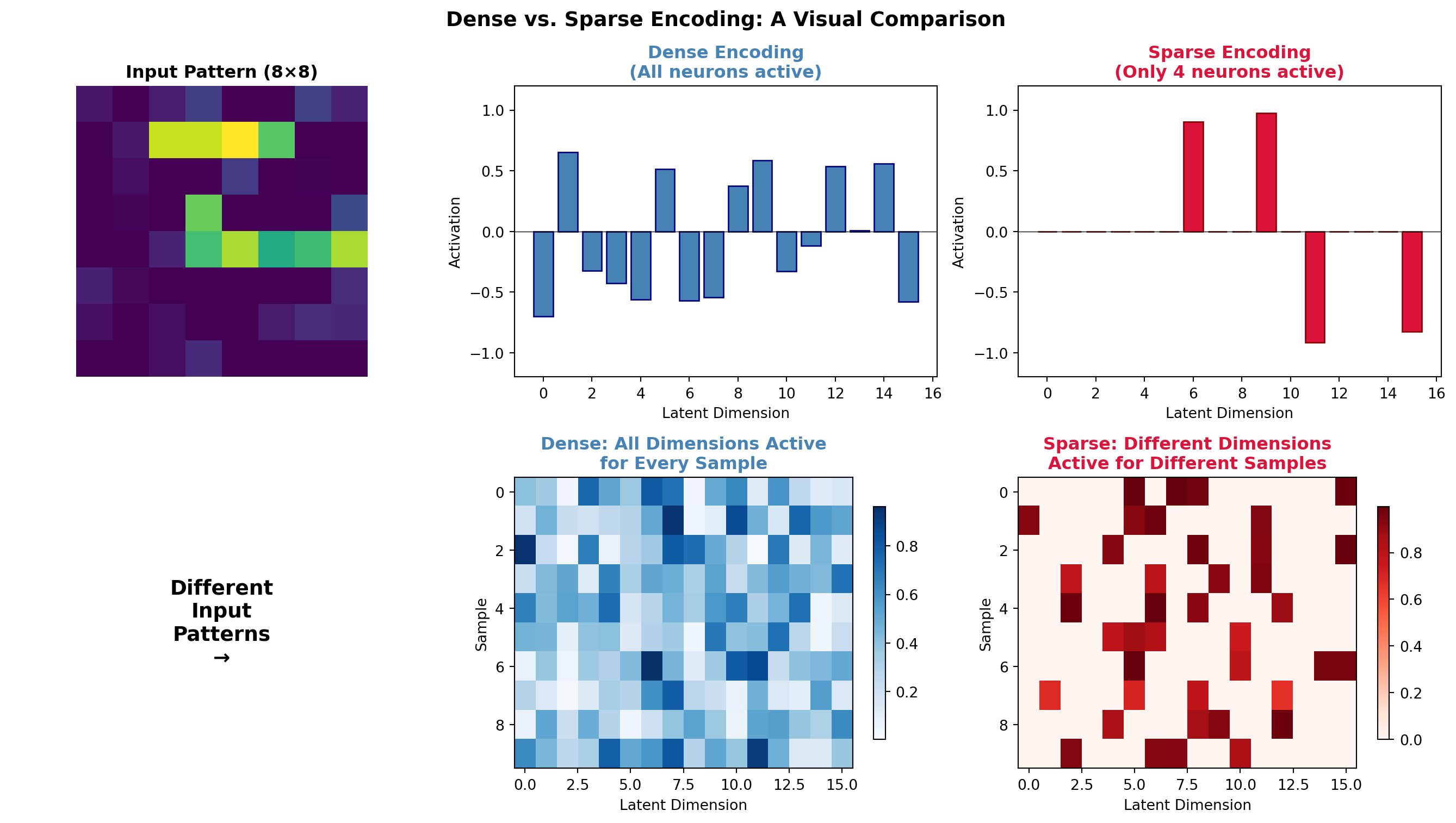
ENCODING STATISTICS
============================================================
Dense encoding - Mean active neurons: 15.9 / 16
Sparse encoding - Mean active neurons: 4.0 / 16

Dense code entropy (information spread): 2.58

Sparse Encoders: The Brain’s Strategy

Sparse encoders create representations where only a small fraction of neurons are active for any given input. This is not just a computational trick. It’s the dominant coding strategy in the brain.

ImportantThe Sparse Coding Hypothesis

In the primary visual cortex (V1), only about 1-5% of neurons are strongly active at any moment, even when viewing complex natural scenes. This sparse, distributed code is metabolically efficient and creates representations that are robust, interpretable, and well-suited for learning.

Olshausen & Field (1996), “Emergence of simple-cell receptive field properties by learning a sparse code for natural images”

Why Sparsity? Three Compelling Reasons:

1. Metabolic Efficiency: Neurons are expensive to fire. Sparse coding minimizes energy use.

2. Increased Capacity: With sparse codes, you can store more patterns without interference. If each pattern activates different neurons, they don’t overwrite each other.

3. Interpretability: When a specific neuron fires, it means something. “Grandmother cells” are an extreme example, but even moderate sparsity creates meaningful selectivity.

Mathematical Formulation:

A sparse autoencoder adds a sparsity penalty to the loss:

\[ \mathcal{L} = \underbrace{\|\mathbf{x} - \hat{\mathbf{x}}\|^2}_{\text{Reconstruction}} + \underbrace{\lambda \sum_j |z_j|}_{\text{L1 Sparsity}} + \underbrace{\beta \sum_j KL(\rho \| \hat{\rho}_j)}_{\text{KL Sparsity (optional)}} \]

Where: - \(\lambda\) controls the strength of L1 regularization (drives activations to exactly zero) - \(\rho\) is the target sparsity (e.g., 0.05 = want 5% average activation) - \(\hat{\rho}_j\) is the actual average activation of neuron \(j\) - \(\beta\) controls KL divergence penalty strength

Types of Sparsity Constraints:

Method	Formula	Effect
L1 Penalty	\(\lambda \sum_j |z_j|\)	Drives small activations to zero
KL Divergence	\(KL(\rho \| \hat{\rho})\)	Controls average activation rate
k-Sparse	Keep top-k, zero rest	Exactly k neurons active
Winner-Take-All	Only max neuron active	Extreme sparsity (k=1)
Lifetime Sparsity	Track usage over time	Each neuron used equally often

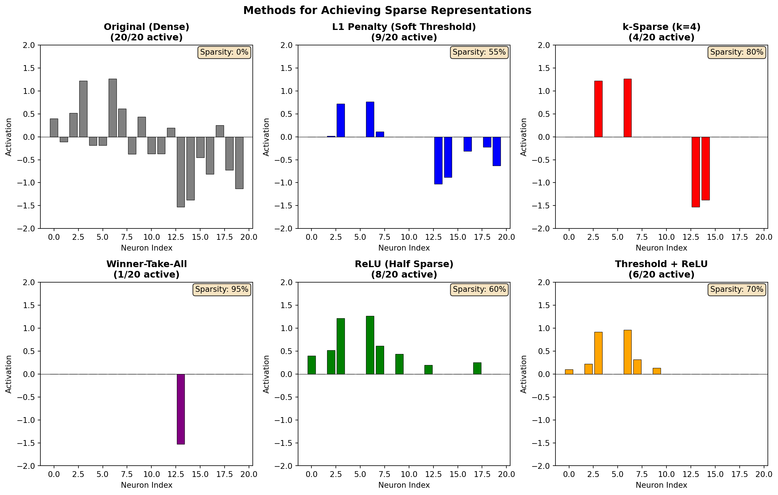
Understanding KL Divergence Sparsity

KL divergence works differently from L1. It controls the average activation rate across a batch of inputs rather than penalizing individual activations.

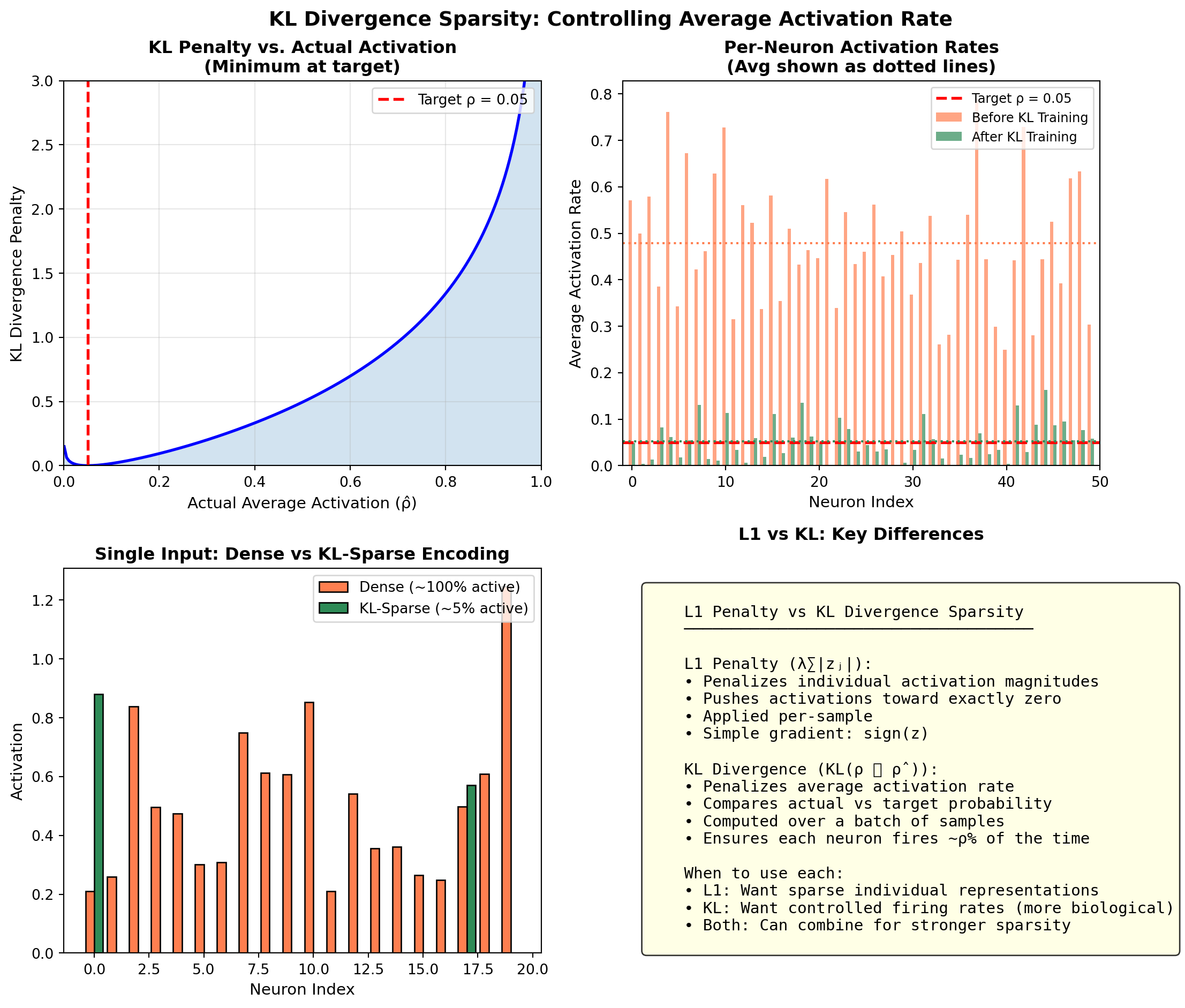
The Neuroscience of Sparse Coding: Lessons from V1

The primary visual cortex (V1) is the brain’s first major visual processing station. Its neurons have become a Rosetta Stone for understanding neural coding.

Key Finding: When Olshausen and Field (1996) trained a sparse autoencoder on natural images, the learned features spontaneously resembled V1 simple cell receptive fields: oriented, localized Gabor-like filters.

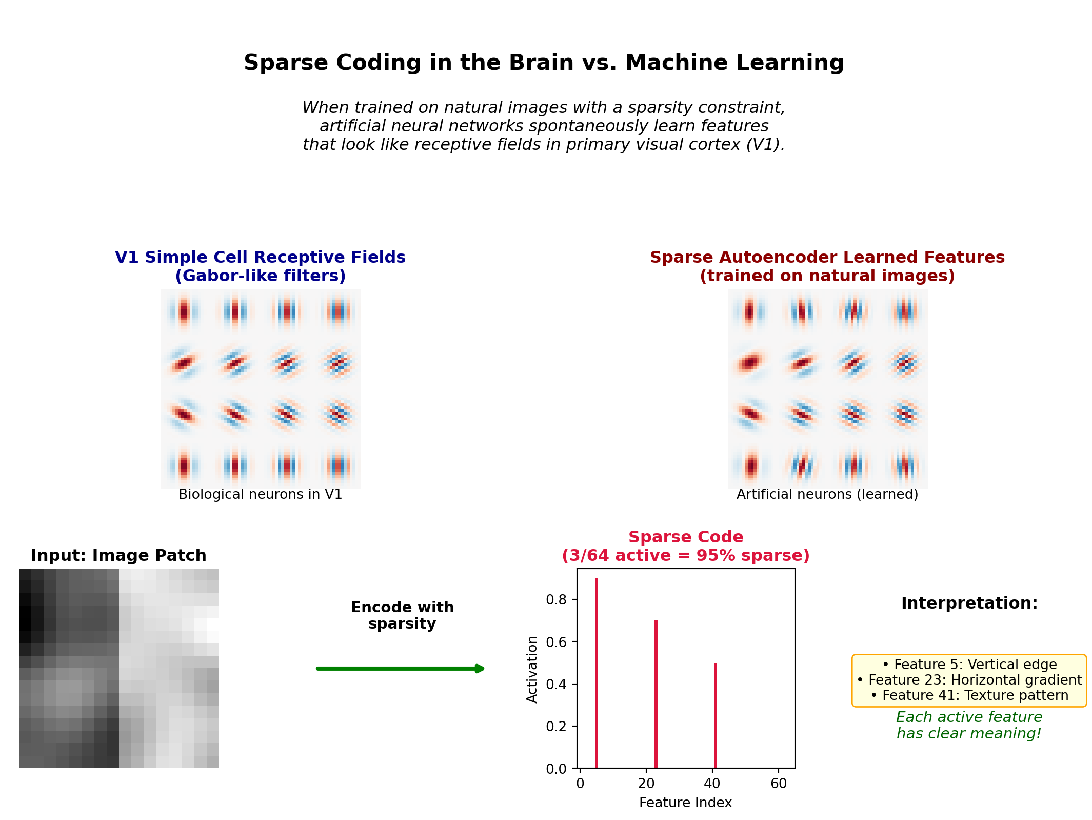
Why Does the Brain Use Sparse Coding?

Reason	Explanation	AI Benefit
Metabolic efficiency	Neurons cost energy; silence is cheap	Lower compute, smaller memory
Storage capacity	Sparse patterns don’t interfere	More patterns stored without overwriting
Fast learning	Few active neurons = credit assignment is easier	Clearer gradients, faster convergence
Robustness	Features are independent; noise affects few	Better generalization
Compositionality	Complex scenes = sum of simple features	Modular, reusable representations

Implementing a Sparse Autoencoder

============================================================
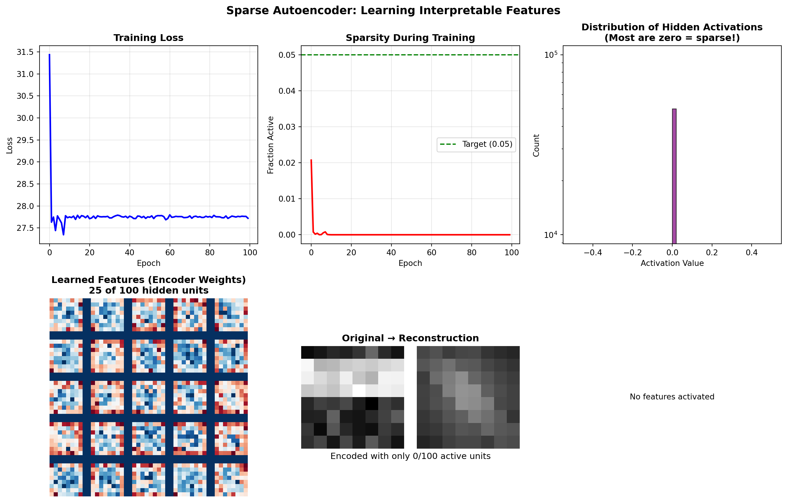
SPARSE AUTOENCODER SUMMARY
============================================================
Architecture: 64 → 100 → 64 (overcomplete)
Final sparsity: 0.0% of neurons active on average
Target sparsity: 5.0%

Dense vs. Sparse: Head-to-Head Comparison

Aspect	Dense Encoder	Sparse Encoder
Architecture	Undercomplete (narrow bottleneck)	Often overcomplete (wide hidden layer)
Activation pattern	All neurons active	Few neurons active (<10%)
Information storage	Distributed holistically	Localized per feature
Interpretability	Low (entangled)	High (each neuron = feature)
Reconstruction	Need all dimensions	Need only active dimensions
Biological analog	Motor cortex, population codes	V1, hippocampus
Training	Standard backprop	Need sparsity regularization
Memory efficiency	Dense activations stored	Only store non-zero indices
Best for	Compression, PCA-like reduction	Feature learning, interpretability

When to Use Which?

TipDecision Guide

Use Dense Encoding when: - Your goal is maximum compression - You have limited latent dimensions - Interpretability doesn’t matter - Downstream task will learn to decode

Use Sparse Encoding when: - You want interpretable features - You need biological plausibility - Memory/compute at inference is limited - You want features that transfer across tasks - Working with high-dimensional overcomplete representations

Code Example: Comparing Dense and Sparse Autoencoders

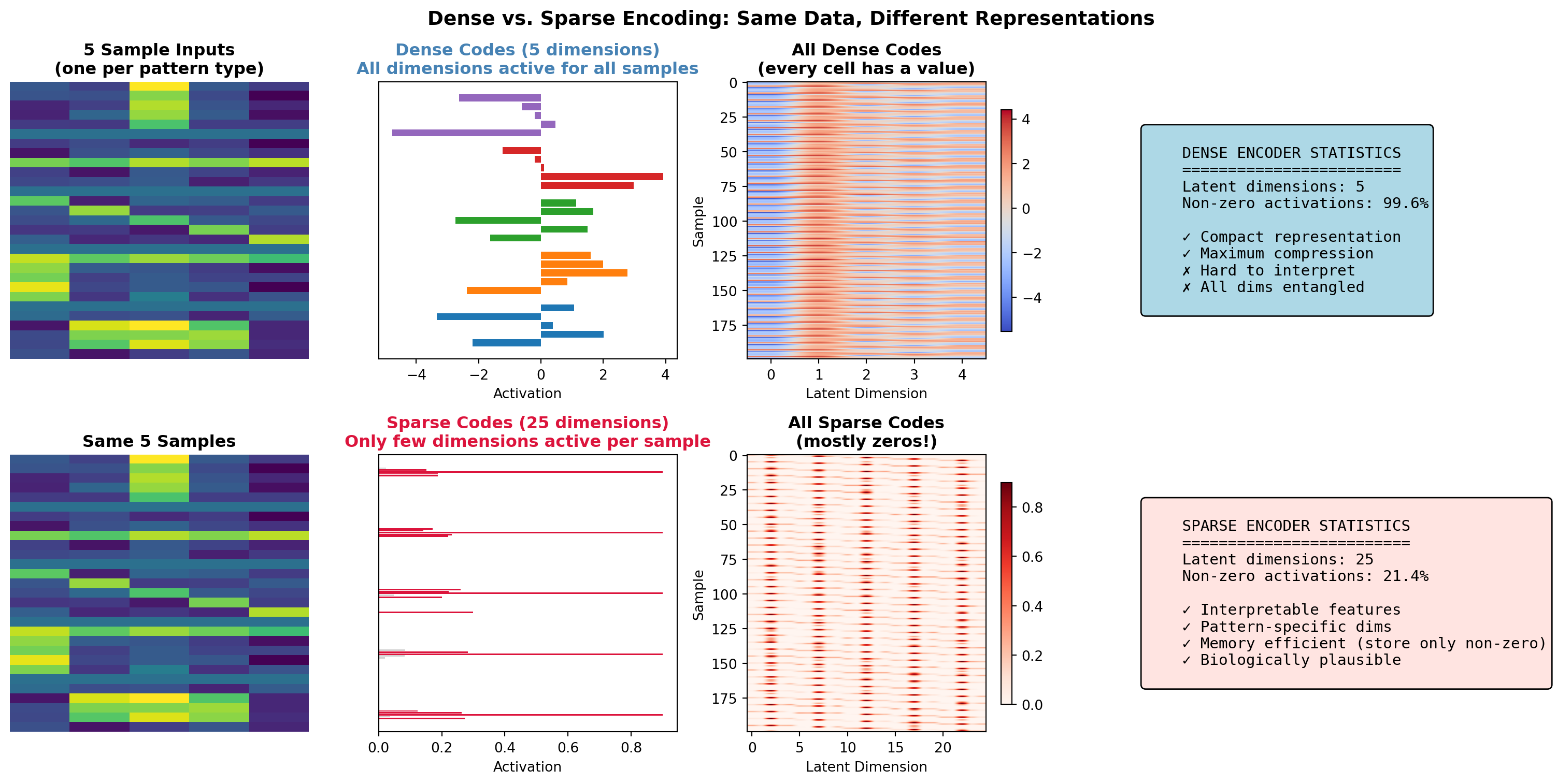
Summary: The Encoding Spectrum

The choice between dense and sparse encoding isn’t binary. It’s a spectrum:

    DENSE                                                      SPARSE
    ←―――――――――――――――――――――――――――――――――――――――――――――――――――――――――→

    PCA    Standard AE    Denoising AE    L1-Sparse AE    k-Sparse    Winner-Take-All

    All neurons          Mild sparsity    Strong sparsity     Only 1 neuron
    active               (dropout helps)   (5-10% active)      active

The brain operates across this spectrum too: - Motor cortex: Dense population codes (all neurons contribute) - V1: Sparse coding (few neurons per stimulus) - Hippocampus: Very sparse (place cells) - Concept neurons: Extremely sparse (grandmother cells?)

Understanding this spectrum is essential for designing neural networks that balance efficiency, interpretability, and biological plausibility.

13.6.4 Variational Autoencoders (VAEs)

VAEs add a probabilistic twist: the encoder outputs parameters of a distribution, not a point:

\[ q_\phi(\mathbf{z}|\mathbf{x}) = \mathcal{N}(\boldsymbol{\mu}_\phi(\mathbf{x}), \boldsymbol{\sigma}^2_\phi(\mathbf{x})) \]

The loss function combines reconstruction and a KL divergence regularizer:

\[ \mathcal{L}_{VAE} = \underbrace{\mathbb{E}_{q}[\log p_\theta(\mathbf{x}|\mathbf{z})]}_{\text{Reconstruction}} - \underbrace{D_{KL}(q_\phi(\mathbf{z}|\mathbf{x}) \| p(\mathbf{z}))}_{\text{Regularization}} \]

The KL term encourages the latent space to be smooth and continuous, enabling generation of new samples.

def vae_latent_space_demo():
    """
    Visualize the difference between AE and VAE latent spaces.
    """
    np.random.seed(42)

    # Simulate latent space samples
    n_samples = 300

    # Standard AE: Clustered, non-continuous latent space
    ae_latent = np.concatenate([
        np.random.randn(100, 2) * 0.3 + np.array([-2, -2]),
        np.random.randn(100, 2) * 0.3 + np.array([2, -2]),
        np.random.randn(100, 2) * 0.3 + np.array([0, 2]),
    ])
    ae_labels = np.concatenate([np.zeros(100), np.ones(100), 2 * np.ones(100)])

    # VAE: Smooth, continuous latent space (approximately Gaussian)
    vae_latent = np.random.randn(n_samples, 2)
    # Color by angle to show structure
    vae_labels = np.arctan2(vae_latent[:, 1], vae_latent[:, 0])

    fig, axes = plt.subplots(1, 2, figsize=(12, 5))

    # AE latent space
    scatter1 = axes[0].scatter(ae_latent[:, 0], ae_latent[:, 1], c=ae_labels, cmap='tab10', s=20, alpha=0.7)
    axes[0].set_title('Standard Autoencoder Latent Space')
    axes[0].set_xlabel('z₁')
    axes[0].set_ylabel('z₂')
    axes[0].annotate('Gaps between\nclusters', xy=(0, 0), fontsize=10,
                     bbox=dict(boxstyle='round', facecolor='wheat', alpha=0.5))

    # VAE latent space
    scatter2 = axes[1].scatter(vae_latent[:, 0], vae_latent[:, 1], c=vae_labels, cmap='hsv', s=20, alpha=0.7)
    axes[1].set_title('VAE Latent Space (KL regularized)')
    axes[1].set_xlabel('z₁')
    axes[1].set_ylabel('z₂')

    # Draw unit circle to show prior
    theta = np.linspace(0, 2 * np.pi, 100)
    axes[1].plot(np.cos(theta), np.sin(theta), 'k--', alpha=0.3, label='Prior N(0,1)')
    axes[1].legend()

    plt.tight_layout()
    return ae_latent, vae_latent

# ae_z, vae_z = vae_latent_space_demo()

13.6.4 The Reparameterization Trick

To backpropagate through stochastic sampling, VAEs use the reparameterization trick:

Instead of sampling \(\mathbf{z} \sim \mathcal{N}(\boldsymbol{\mu}, \boldsymbol{\sigma}^2)\), we compute: \[ \mathbf{z} = \boldsymbol{\mu} + \boldsymbol{\sigma} \odot \boldsymbol{\epsilon}, \quad \boldsymbol{\epsilon} \sim \mathcal{N}(0, \mathbf{I}) \]

This moves the stochasticity outside the computational graph, enabling standard backpropagation.

13.6.5 Neuroscience Connections

Autoencoders have profound connections to brain computation:

Autoencoder Concept	Brain Analog
Bottleneck compression	Efficient coding (Ch 7)
Sparse coding	V1 sparse representations
Reconstruction	Predictive coding top-down predictions
Latent space	Neural manifolds
Denoising	Robust sensory processing
Hierarchical AE	Cortical hierarchy

TipThe Information Bottleneck View

Autoencoders implement the information bottleneck principle: compress the input while preserving information relevant for reconstruction. This is precisely what the brain must do: compress high-dimensional sensory data into low-dimensional neural codes while preserving behaviorally relevant information. See Chapter 7 for the information-theoretic foundations.

13.6.6 Code Lab: Building a VAE

def build_vae_conceptual():
    """
    Conceptual implementation of a VAE architecture.
    (Full implementation would use PyTorch/TensorFlow)
    """
    # Architecture diagram
    architecture = """
    VAE Architecture:

    INPUT (x)
       │
       ▼
    ┌─────────┐
    │ ENCODER │ (neural network)
    └────┬────┘
         │
    ┌────┴────┐
    │    │    │
    ▼    ▼    ▼
    μ    σ    (parameters of q(z|x))
    │    │
    └─┬──┘
      │ z = μ + σ * ε  (reparameterization)
      │ ε ~ N(0, I)
      ▼
    ┌─────────┐
    │ DECODER │ (neural network)
    └────┬────┘
         │
         ▼
    OUTPUT (x̂)

    Loss = Reconstruction + β * KL(q(z|x) || p(z))
    """
    print(architecture)

    # Demonstrate the loss components
    def vae_loss_components(x, x_recon, mu, log_var, beta=1.0):
        """
        Compute VAE loss components.

        Args:
            x: Original input
            x_recon: Reconstructed input
            mu: Mean of latent distribution
            log_var: Log variance of latent distribution
            beta: Weight on KL term (beta-VAE)
        """
        # Reconstruction loss (MSE or BCE depending on data)
        recon_loss = np.mean((x - x_recon) ** 2)

        # KL divergence: D_KL(N(μ, σ²) || N(0, 1))
        # = -0.5 * Σ(1 + log(σ²) - μ² - σ²)
        kl_loss = -0.5 * np.mean(1 + log_var - mu ** 2 - np.exp(log_var))

        total_loss = recon_loss + beta * kl_loss

        return {
            'reconstruction': recon_loss,
            'kl_divergence': kl_loss,
            'total': total_loss,
            'beta': beta
        }

    # Example
    np.random.seed(42)
    x = np.random.randn(32, 784)  # Batch of 32 MNIST-like images
    x_recon = x + np.random.randn(32, 784) * 0.1  # Noisy reconstruction
    mu = np.random.randn(32, 20) * 0.5  # 20-dim latent
    log_var = np.random.randn(32, 20) * 0.1 - 1

    losses = vae_loss_components(x, x_recon, mu, log_var, beta=1.0)
    print("\nVAE Loss Components:")
    print(f"  Reconstruction Loss: {losses['reconstruction']:.4f}")
    print(f"  KL Divergence:       {losses['kl_divergence']:.4f}")
    print(f"  Total Loss (β={losses['beta']}): {losses['total']:.4f}")

    return losses

# losses = build_vae_conceptual()

13.6.7 Applications of Autoencoders

1. Dimensionality Reduction: Nonlinear alternative to PCA
2. Anomaly Detection: High reconstruction error indicates anomalies
3. Denoising: Learn to remove noise from corrupted inputs
4. Generative Modeling: VAEs can generate new samples
5. Representation Learning: Pre-train encoders for downstream tasks
6. Neural Data Analysis: Discover latent structure in neural recordings (Ch 24)

20.8 13.7 Code Lab: Implementing a Neural Network from Scratch

Let’s implement a simple neural network without using deep learning frameworks to understand the core concepts better:

def neural_network_from_scratch():
    """Implement a simple neural network from scratch."""
    # Define network architecture
    input_size = 2
    hidden_size = 3
    output_size = 1
    
    # Generate synthetic data
    np.random.seed(42)
    X = np.random.randn(100, input_size)
    # True function: XOR-like (non-linear)
    y = np.array([(x[0] > 0) != (x[1] > 0) for x in X]).reshape(-1, 1).astype(float)
    
    # Initialize weights and biases
    def init_params():
        np.random.seed(42)
        W1 = np.random.randn(input_size, hidden_size) * 0.1
        b1 = np.zeros((1, hidden_size))
        W2 = np.random.randn(hidden_size, output_size) * 0.1
        b2 = np.zeros((1, output_size))
        return {'W1': W1, 'b1': b1, 'W2': W2, 'b2': b2}
    
    # Activation functions
    def sigmoid(x):
        return 1 / (1 + np.exp(-x))
    
    def sigmoid_derivative(x):
        s = sigmoid(x)
        return s * (1 - s)
    
    # Forward pass
    def forward(X, params):
        W1, b1, W2, b2 = params['W1'], params['b1'], params['W2'], params['b2']
        
        # Hidden layer
        Z1 = X @ W1 + b1
        A1 = sigmoid(Z1)
        
        # Output layer
        Z2 = A1 @ W2 + b2
        A2 = sigmoid(Z2)
        
        cache = {'Z1': Z1, 'A1': A1, 'Z2': Z2, 'A2': A2, 'X': X}
        return A2, cache
    
    # Compute loss
    def compute_loss(A2, y):
        m = y.shape[0]
        loss = -np.sum(y * np.log(A2 + 1e-8) + (1 - y) * np.log(1 - A2 + 1e-8)) / m
        return loss
    
    # Backward pass
    def backward(cache, y, params):
        m = y.shape[0]
        W1, W2 = params['W1'], params['W2']
        A1, A2 = cache['A1'], cache['A2']
        X = cache['X']
        
        # Output layer
        dZ2 = A2 - y
        dW2 = A1.T @ dZ2 / m
        db2 = np.sum(dZ2, axis=0, keepdims=True) / m
        
        # Hidden layer
        dA1 = dZ2 @ W2.T
        dZ1 = dA1 * sigmoid_derivative(cache['Z1'])
        dW1 = X.T @ dZ1 / m
        db1 = np.sum(dZ1, axis=0, keepdims=True) / m
        
        gradients = {'dW1': dW1, 'db1': db1, 'dW2': dW2, 'db2': db2}
        return gradients
    
    # Update parameters
    def update_params(params, gradients, learning_rate):
        params['W1'] -= learning_rate * gradients['dW1']
        params['b1'] -= learning_rate * gradients['db1']
        params['W2'] -= learning_rate * gradients['dW2']
        params['b2'] -= learning_rate * gradients['db2']
        return params
    
    # Training loop
    def train(X, y, hidden_size, learning_rate, epochs):
        # Initialize parameters
        params = init_params()
        
        # Track loss
        losses = []
        
        # Training iterations
        for i in range(epochs):
            # Forward pass
            A2, cache = forward(X, params)
            
            # Compute loss
            loss = compute_loss(A2, y)
            losses.append(loss)
            
            # Backward pass
            gradients = backward(cache, y, params)
            
            # Update parameters
            params = update_params(params, gradients, learning_rate)
            
            # Print loss every 1000 epochs
            if i % 1000 == 0:
                print(f"Epoch {i}, Loss: {loss:.4f}")
        
        return params, losses
    
    # Train the network
    params, losses = train(X, y, hidden_size, learning_rate=0.5, epochs=5000)
    
    # Visualize the results
    def visualize_results():
        # Visualization of training progress
        plt.figure(figsize=(12, 5))
        
        # Loss curve
        plt.subplot(1, 2, 1)
        plt.plot(losses)
        plt.title('Training Loss')
        plt.xlabel('Epoch')
        plt.ylabel('Loss')
        plt.grid(True)
        
        # Decision boundary
        plt.subplot(1, 2, 2)
        
        # Create a mesh grid
        h = 0.01
        x_min, x_max = X[:, 0].min() - 1, X[:, 0].max() + 1
        y_min, y_max = X[:, 1].min() - 1, X[:, 1].max() + 1
        xx, yy = np.meshgrid(np.arange(x_min, x_max, h),
                             np.arange(y_min, y_max, h))
        
        # Make predictions on the mesh grid
        Z, _ = forward(np.c_[xx.ravel(), yy.ravel()], params)
        Z = Z.reshape(xx.shape)
        
        # Plot decision boundary
        plt.contourf(xx, yy, Z, cmap=plt.cm.Spectral, alpha=0.8)
        
        # Plot training examples
        plt.scatter(X[:, 0], X[:, 1], c=y.ravel(), cmap=plt.cm.Spectral, edgecolors='k')
        plt.title('Decision Boundary')
        plt.xlabel('Feature 1')
        plt.ylabel('Feature 2')
        
        plt.tight_layout()
        return plt
    
    return visualize_results()

This implementation demonstrates the core components of neural networks:

1. Forward Propagation: Computing activations through the network
2. Loss Calculation: Measuring how far predictions are from targets
3. Backward Propagation: Computing gradients for each parameter
4. Parameter Updates: Adjusting weights and biases using gradients

While modern deep learning frameworks automate these steps, understanding the underlying mechanics is crucial for debugging, customization, and optimization.

20.9 13.8 Take-aways

• Framework Abstraction: Modern deep learning frameworks like PyTorch and TensorFlow abstract low-level details, allowing researchers to focus on architecture design and experimentation.

• Training Stability: Achieving stable training requires careful attention to initialization, normalization, learning rates, and gradient flow.

• Regularization Importance: Regularization techniques critically impact model generalization, with techniques like dropout, batch normalization, and weight decay combining for best results.

• Architectural Innovations: Advances like residual connections enable training of extremely deep networks by mitigating gradient flow issues.

• Optimization Challenges: Deep learning optimization remains challenging due to non-convex loss landscapes, saddle points, and the need to escape poor local minima.

• Empirical Focus: Despite theoretical progress, deep learning remains heavily empirical, with practical techniques often preceding theoretical understanding.

```zbtgbcnjthwwyc: Chapter Summary :class: important

In this chapter, we explored:

• Neural network fundamentals including multilayer perceptrons and the mathematics of backpropagation
• Activation functions from sigmoid and tanh to modern variants like ReLU, GELU, and Swish
• The vanishing/exploding gradient problem and techniques to address it
• Optimization algorithms such as SGD, momentum, Adam, and second-order methods
• Learning rate scheduling approaches that adapt optimization dynamics during training
• Regularization techniques including dropout, batch normalization, and weight decay
• Advanced architectures like convolutional neural networks, residual networks, and graph neural networks
• Biological parallels between deep learning systems and neural computations in the brain
• Modern paradigms such as self-supervised learning and foundation models
• Theoretical frameworks including loss landscapes, generalization theory, and neural tangent kernels

This chapter provides a comprehensive overview of deep learning fundamentals, from the mathematical principles that enable training to practical techniques that improve performance, while highlighting both the technological innovations and biological inspirations that shape modern neural networks.

```{"admonition"}: Knowledge Connections
:class: important

**Looking Back**
- **Chapter 1 (Introduction)**: The backpropagation algorithm introduced in section 1.1.3 is explored in depth here, showing how it enables training of complex neural networks.
- **Chapter 2 (Neuroscience Foundations)**: The biological learning mechanisms described in section 2.3 provide an interesting contrast to the optimization algorithms covered in this chapter.
- **Chapter 7 (Information Theory)**: The information bottleneck principle (section 7.6) provides theoretical insights into how deep networks compress information through layers.
- **Chapter 9 (ML Foundations)**: The basic learning algorithms from Chapter 9 are extended here to handle deep architectures and large-scale training.

**Looking Forward**
- **Chapter 11 (Sequence Models)**: The optimization techniques learned here will be applied to the specialized architectures for sequential data.
- **Chapter 12 (Large Language Models)**: The scaling laws and foundation model concepts introduced in section 13.6.2 become critical for understanding LLM training and capabilities.
- **Chapter 14 (Future Directions)**: The biological parallels in deep learning (section 13.5) point to neuromorphic approaches that may shape future AI systems.

20.10 13.9 Exercises

Conceptual Questions

1. Explain the vanishing and exploding gradient problems in deep networks. Why do these problems occur during backpropagation through many layers? How do modern techniques like residual connections, batch normalization, and careful initialization help mitigate these issues?

2. Compare different activation functions and their properties. For each of ReLU, sigmoid, tanh, and variants (Leaky ReLU, ELU, Swish):

   • Describe the function mathematically
   • Explain when it saturates (if at all)
   • Discuss its gradient properties
   • Provide use cases where it’s preferred

3. Explain the bias-variance trade-off in deep learning. How do deep networks with millions of parameters avoid overfitting despite classical statistical theory suggesting they should? Discuss the roles of implicit regularization in SGD, dropout, data augmentation, and the double descent phenomenon.

4. Describe the function of batch normalization beyond just normalization. Beyond reducing internal covariate shift, what other effects does batch normalization have on the loss landscape smoothness, learning rate sensitivity, gradient flow, and implicit regularization?

Computational Exercises

5. Implement backpropagation from scratch. Write code to:
   • Build a simple feedforward network without using autograd
   • Manually implement forward and backward passes for linear and ReLU layers
   • Compute gradients using the chain rule
   • Train on a simple dataset (e.g., XOR or MNIST)
   • Verify your gradients using numerical differentiation
   • Compare performance to a framework implementation (PyTorch/TensorFlow)
6. Analyze the effect of network depth. Implement:
   • Networks with 2, 5, 10, and 20 layers on the same task
   • Measure: training time, convergence speed, final test accuracy
   • Visualize gradient magnitudes at different layers during training
   • Add residual connections to the deep network and compare results
   • Discuss the empirical benefits and costs of depth
7. Compare optimization algorithms. Implement and compare:
   • SGD, SGD with momentum, RMSProp, Adam
   • Use the same network architecture and dataset
   • Plot loss curves, learning rate schedules, and convergence speed
   • Measure sensitivity to learning rate choice for each
   • Discuss when you would prefer each optimizer
8. Investigate regularization techniques. Create:
   • A network prone to overfitting (large capacity, small dataset)
   • Compare: no regularization, L2 regularization, dropout, data augmentation, early stopping
   • Plot training vs. validation curves for each
   • Measure the test accuracy for each method
   • Combine multiple techniques and analyze the effect

Discussion Questions

9. Deep learning and biological plausibility. Discuss:
   • What aspects of backpropagation are biologically implausible (weight symmetry, separate forward/backward passes, etc.)?
   • What are alternative learning algorithms that are more biologically plausible (e.g., feedback alignment, target propagation)?
   • Do biological plausibility constraints matter for AI performance, or only for understanding the brain?
   • Could insights from neuroscience lead to better training algorithms for deep networks?
10. The future of deep learning architectures. Consider:
    • Are we approaching the limits of what can be achieved by scaling current architectures?
    • What role will inductive biases (like convolution, attention) play versus fully general architectures?
    • How might sparsity (in activations, weights, or gradients) change deep learning?
    • What are the next frontiers: multimodal models, continual learning, energy efficiency, or something else?
11. Ethics and environmental impact of deep learning. Reflect on:
    • The carbon footprint of training large models and how to mitigate it
    • The trade-off between model performance and environmental cost
    • Whether the democratization of AI is helped or hindered by the trend toward larger models
    • How research priorities should balance pushing capabilities forward with efficiency and accessibility

20.11 13.10 References

• Goodfellow, I., Bengio, Y., & Courville, A. (2016). Deep Learning. MIT Press.

• LeCun, Y., Bengio, Y., & Hinton, G. (2015). Deep learning. Nature, 521(7553), 436-444.

• Krizhevsky, A., Sutskever, I., & Hinton, G. E. (2012). ImageNet classification with deep convolutional neural networks. Advances in Neural Information Processing Systems, 25, 1097-1105.

• He, K., Zhang, X., Ren, S., & Sun, J. (2016). Deep residual learning for image recognition. IEEE Conference on Computer Vision and Pattern Recognition, 770-778.

• Kingma, D. P., & Ba, J. (2015). Adam: A method for stochastic optimization. International Conference on Learning Representations.

• Ioffe, S., & Szegedy, C. (2015). Batch normalization: Accelerating deep network training by reducing internal covariate shift. International Conference on Machine Learning, 448-456.

• Srivastava, N., Hinton, G., Krizhevsky, A., Sutskever, I., & Salakhutdinov, R. (2014). Dropout: A simple way to prevent neural networks from overfitting. Journal of Machine Learning Research, 15(1), 1929-1958.

• Vaswani, A., Shazeer, N., Parmar, N., Uszkoreit, J., Jones, L., Gomez, A. N., et al. (2017). Attention is all you need. Advances in Neural Information Processing Systems, 30, 5998-6008.

• Smith, L. N. (2018). A disciplined approach to neural network hyper-parameters: Part 1 - learning rate, batch size, momentum, and weight decay. arXiv preprint arXiv:1803.09820.

• Zhang, C., Bengio, S., Hardt, M., Recht, B., & Vinyals, O. (2021). Understanding deep learning (still) requires rethinking generalization. Communications of the ACM, 64(3), 107-115.

• Li, H., Xu, Z., Taylor, G., Studer, C., & Goldstein, T. (2018). Visualizing the loss landscape of neural nets. Advances in Neural Information Processing Systems, 31, 6389-6399.

• Jacot, A., Gabriel, F., & Hongler, C. (2018). Neural tangent kernel: Convergence and generalization in neural networks. Advances in Neural Information Processing Systems, 31, 8571-8580.