2 Lab 2: Neuroscience Foundations for AI

2.1 Learning Objectives
By the end of this lab, you will be able to:
- Implement a leaky integrate-and-fire (LIF) neuron model with refractory periods
- Simulate spiking neural networks with excitatory and inhibitory neurons
- Apply spike-timing-dependent plasticity (STDP) to model synaptic learning
- Implement homeostatic mechanisms for network stability
- Visualize neural activity patterns, weight dynamics, and firing rate regulation
2.2 Prerequisites
- Reading: Chapter 2: Neuroscience Foundations for AI
- Libraries: NumPy, Matplotlib
- Concepts: Differential equations, neural dynamics, synaptic plasticity
2.3 Setup
import numpy as np
import matplotlib.pyplot as plt

## Set random seed for reproducibility
np.random.seed(42)
rng = np.random.default_rng(42)

## Set plotting style
plt.style.use('default')
plt.rcParams['figure.figsize'] = (12, 8)
plt.rcParams['font.size'] = 11
2.4 Part 1: Single Leaky Integrate-and-Fire (LIF) Neuron
2.4.1 1.1 Understanding the LIF Model
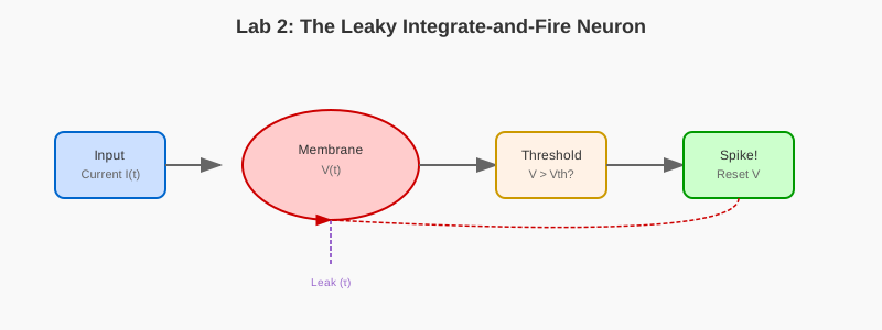
The LIF neuron is a simple but powerful model that captures key features of biological neurons: - Leak: Membrane potential decays toward rest - Integration: Incoming currents charge the membrane - Fire: When voltage crosses threshold, emit a spike - Reset: Return to reset potential after spiking
Key Equation: \[\tau_m \frac{dV}{dt} = -(V - V_{rest}) + R_m I(t)\]
Where: - \(V\): membrane potential - \(\tau_m\): membrane time constant - \(V_{rest}\): resting potential - \(R_m\): membrane resistance - \(I(t)\): input current
def simulate_lif_neuron(I_ext, T_ms=500, dt=0.1, V_rest=-70, V_thresh=-50,
                       V_reset=-65, tau_m=20, R_m=10, t_ref=3):
    """
    Simulate a single LIF neuron with refractory period.

    Args:
        I_ext: External current (array or constant)
        T_ms: Simulation time in milliseconds
        dt: Time step in ms
        V_rest: Resting potential (mV)
        V_thresh: Spike threshold (mV)
        V_reset: Reset potential (mV)
        tau_m: Membrane time constant (ms)
        R_m: Membrane resistance (MOhm)
        t_ref: Refractory period (ms)

    Returns:
        time, voltage trace, spike times
    """
    steps = int(T_ms / dt)
    time = np.arange(steps) * dt
    V = np.zeros(steps)
    V[0] = V_rest
    spikes = []
    refrac_until = 0  # Time until which neuron is refractory

    # Make I_ext an array if it's a scalar
    if np.isscalar(I_ext):
        I_ext = np.full(steps, I_ext)

    for t in range(1, steps):
        if time[t] < refrac_until:
            # Neuron is refractory, clamp voltage
            V[t] = V_reset
        else:
            # Update voltage using Euler method
            dV = (-(V[t-1] - V_rest) + R_m * I_ext[t-1]) / tau_m
            V[t] = V[t-1] + dt * dV

            # Check for threshold crossing
            if V[t] >= V_thresh:
                spikes.append(time[t])
                V[t] = V_reset
                refrac_until = time[t] + t_ref

    return time, V, np.array(spikes)

## Example 1: Constant input
I_constant = 2.5  # nA
time, V, spikes = simulate_lif_neuron(I_constant, T_ms=200)

## Plot
fig, (ax1, ax2) = plt.subplots(2, 1, figsize=(12, 8))

ax1.plot(time, V, linewidth=2, color='#cc0000')
ax1.axhline(y=-50, color='gray', linestyle='--', label='Threshold')
ax1.axhline(y=-70, color='lightgray', linestyle='--', label='Rest')
ax1.set_ylabel('Voltage (mV)', fontsize=12)
ax1.set_title('LIF Neuron with Constant Input', fontsize=14, fontweight='bold')
ax1.legend()
ax1.grid(True, alpha=0.3)

ax2.plot(time, [I_constant] * len(time), linewidth=2, color='#0066cc')
ax2.set_xlabel('Time (ms)', fontsize=12)
ax2.set_ylabel('Input Current (nA)', fontsize=12)
ax2.set_title('Input Current', fontsize=12)
ax2.grid(True, alpha=0.3)

plt.tight_layout()
plt.show()

print(f\"Number of spikes: {len(spikes)}\")
print(f\"Firing rate: {len(spikes) / (time[-1]/1000):.2f} Hz\")
2.4.2 1.2 Response to Different Input Patterns
## Generate different input patterns
T_ms = 500
dt = 0.1
steps = int(T_ms / dt)
time = np.arange(steps) * dt

## Pattern 1: Step input
I_step = np.zeros(steps)
I_step[1000:4000] = 3.0

## Pattern 2: Ramp input
I_ramp = np.linspace(0, 4, steps)

## Pattern 3: Oscillating input
I_osc = 2.0 + 1.5 * np.sin(2 * np.pi * 0.01 * time)

## Pattern 4: Noisy input
I_noisy = 2.5 + 0.5 * np.random.randn(steps)

## Simulate all patterns
patterns = {
    'Step': I_step,
    'Ramp': I_ramp,
    'Oscillating': I_osc,
    'Noisy': I_noisy
}

fig, axes = plt.subplots(4, 2, figsize=(14, 12))

for idx, (name, I_pattern) in enumerate(patterns.items()):
    _, V, spikes = simulate_lif_neuron(I_pattern, T_ms=T_ms, dt=dt)

    # Plot voltage
    axes[idx, 0].plot(time, V, linewidth=1.5, color='#cc0000')
    axes[idx, 0].axhline(y=-50, color='gray', linestyle='--', alpha=0.5)
    axes[idx, 0].set_ylabel('V (mV)')
    axes[idx, 0].set_title(f'{name} Input - Voltage Response', fontweight='bold')
    axes[idx, 0].grid(True, alpha=0.3)

    # Plot input
    axes[idx, 1].plot(time, I_pattern, linewidth=1.5, color='#0066cc')
    axes[idx, 1].set_ylabel('I (nA)')
    axes[idx, 1].set_title(f'{name} Input Current', fontweight='bold')
    axes[idx, 1].grid(True, alpha=0.3)

    if idx == 3:
        axes[idx, 0].set_xlabel('Time (ms)')
        axes[idx, 1].set_xlabel('Time (ms)')

    print(f\"{name}: {len(spikes)} spikes, {len(spikes)/(T_ms/1000):.1f} Hz\")

plt.tight_layout()
plt.show()
Exercise 1.1: What is the minimum constant current needed to make the neuron spike? (Hint: Try values from 1.0 to 3.0 nA and plot firing rate vs. current)
Exercise 1.2: How does the refractory period affect maximum firing rate? Set t_ref to [1, 3, 5, 10] ms and measure maximum achievable firing rate with strong input.
2.5 Part 2: Network of LIF Neurons
2.5.1 2.1 Implementing a Spiking Network
Now let’s scale up to a population of interconnected neurons with both excitatory and inhibitory cells.
def simulate_lif_network(N=100, frac_exc=0.8, T_ms=1000, dt=0.5,
                        ext_rate_hz=5.0, ext_I_amp=1.2):
    \"\"\"
    Simulate a network of LIF neurons with E/I balance.

    Args:
        N: Number of neurons
        frac_exc: Fraction of excitatory neurons
        T_ms: Simulation time (ms)
        dt: Time step (ms)
        ext_rate_hz: External Poisson input rate (Hz)
        ext_I_amp: External input amplitude

    Returns:
        time, spike_train, weight_matrix
    \"\"\"
    steps = int(T_ms / dt)
    time = np.arange(steps) * dt

    # Neuron populations
    Ne = int(N * frac_exc)
    Ni = N - Ne
    exc_idx = np.arange(Ne)
    inh_idx = np.arange(Ne, N)

    # Neuron parameters
    V_rest = -70.0
    V_reset = -65.0
    V_thresh = -50.0
    tau_m = np.full(N, 20.0)
    R_m = np.full(N, 10.0)
    t_ref = np.full(N, 3.0)
    refrac_until = np.zeros(N)

    # Initialize weights: E->* positive, I->* negative
    W = rng.normal(0.0, 0.05, size=(N, N))
    W[:, inh_idx] = -np.abs(W[:, inh_idx])  # Inhibitory weights negative
    W[:, exc_idx] = np.abs(W[:, exc_idx])   # Excitatory weights positive
    np.fill_diagonal(W, 0.0)

    # Clip weights to reasonable ranges
    W[:, exc_idx] = np.clip(W[:, exc_idx], 0.0, 0.5)
    W[:, inh_idx] = np.clip(W[:, inh_idx], -1.0, 0.0)

    # External Poisson input (to E neurons only)
    ext_spikes = rng.random((steps, Ne)) < (ext_rate_hz * dt / 1000.0)

    # State variables
    V = np.full(N, V_rest)
    spike_train = np.zeros((steps, N), dtype=bool)

    # Simulation loop
    for t in range(steps):
        # External current
        I_ext = np.zeros(N)
        I_ext[exc_idx] = ext_I_amp * ext_spikes[t].astype(float)

        # Synaptic current from network
        if t > 0:
            I_syn = W @ spike_train[t-1].astype(float)
        else:
            I_syn = np.zeros(N)

        # Update voltage
        dV = (-(V - V_rest) + R_m * (I_ext + I_syn)) / tau_m
        V = V + dt * dV

        # Clamp refractory neurons
        V[time[t] < refrac_until] = V_reset

        # Check threshold
        spk = (V >= V_thresh)
        spike_train[t, spk] = True
        V[spk] = V_reset
        refrac_until[spk] = time[t] + t_ref[spk]

    return time, spike_train, W

## Simulate network
time, spikes, W = simulate_lif_network(N=100, T_ms=1000)

## Visualize
fig, axes = plt.subplots(2, 2, figsize=(14, 10))

## Raster plot
ax = axes[0, 0]
N = spikes.shape[1]
for i in range(N):
    spike_times = time[spikes[:, i]]
    ax.vlines(spike_times, i+0.5, i+1.5, color='k', linewidth=0.5)
ax.set_xlim(0, time[-1])
ax.set_ylim(0.5, N+0.5)
ax.set_xlabel('Time (ms)')
ax.set_ylabel('Neuron Index')
ax.set_title('Network Spike Raster', fontweight='bold')
ax.axhline(y=80, color='red', linestyle='--', alpha=0.5, label='E/I boundary')
ax.legend()

## Population firing rates
ax = axes[0, 1]
window = 50  # ms
win_steps = int(window / 0.5)
exc_rate = []
inh_rate = []
time_bins = []

for t in range(0, len(time) - win_steps, win_steps // 2):
    exc_spikes = spikes[t:t+win_steps, :80].sum()
    inh_spikes = spikes[t:t+win_steps, 80:].sum()
    exc_rate.append(exc_spikes / (80 * window / 1000))
    inh_rate.append(inh_spikes / (20 * window / 1000))
    time_bins.append(time[t + win_steps // 2])

ax.plot(time_bins, exc_rate, label='Excitatory', linewidth=2, color='#cc0000')
ax.plot(time_bins, inh_rate, label='Inhibitory', linewidth=2, color='#0066cc')
ax.set_xlabel('Time (ms)')
ax.set_ylabel('Firing Rate (Hz)')
ax.set_title('Population Firing Rates', fontweight='bold')
ax.legend()
ax.grid(True, alpha=0.3)

## Weight matrix
ax = axes[1, 0]
im = ax.imshow(W, aspect='auto', cmap='RdBu_r', vmin=-1, vmax=1)
ax.set_title('Weight Matrix', fontweight='bold')
ax.set_xlabel('Presynaptic Neuron')
ax.set_ylabel('Postsynaptic Neuron')
plt.colorbar(im, ax=ax, label='Weight')

## Firing rate distribution
ax = axes[1, 1]
firing_rates = spikes.sum(axis=0) / (time[-1] / 1000)
ax.hist(firing_rates[:80], bins=20, alpha=0.7, label='Excitatory', color='#cc0000')
ax.hist(firing_rates[80:], bins=20, alpha=0.7, label='Inhibitory', color='#0066cc')
ax.set_xlabel('Firing Rate (Hz)')
ax.set_ylabel('Count')
ax.set_title('Firing Rate Distribution', fontweight='bold')
ax.legend()
ax.grid(True, alpha=0.3)

plt.tight_layout()
plt.show()

print(f\"Mean E firing rate: {firing_rates[:80].mean():.2f} ± {firing_rates[:80].std():.2f} Hz\")
print(f\"Mean I firing rate: {firing_rates[80:].mean():.2f} ± {firing_rates[80:].std():.2f} Hz\")
Exercise 2.1: Vary the E/I ratio (frac_exc from 0.5 to 0.9). How does this affect network dynamics and firing rates?
Exercise 2.2: What happens when you remove all inhibition (set all I->E weights to 0)? Does the network become unstable?
2.6 Part 3: Spike-Timing-Dependent Plasticity (STDP)
2.6.1 3.1 Understanding STDP
STDP implements Hebb’s rule with a temporal component: - Pre before Post (causality): Strengthen synapse (LTP) - Post before Pre (anti-causality): Weaken synapse (LTD)
This allows the network to learn temporal relationships and causal structure.
def stdp_weight_change(dt, tau_plus=20, tau_minus=20, A_plus=0.01, A_minus=-0.01):
    \"\"\"
    Calculate STDP weight change based on spike timing.

    Args:
        dt: Time difference (post_time - pre_time) in ms
        tau_plus: Time constant for LTP (ms)
        tau_minus: Time constant for LTD (ms)
        A_plus: LTP amplitude
        A_minus: LTD amplitude

    Returns:
        Weight change
    \"\"\"
    if dt > 0:
        # Post after pre: LTP
        return A_plus * np.exp(-dt / tau_plus)
    else:
        # Pre after post: LTD
        return A_minus * np.exp(dt / tau_minus)

## Visualize STDP curve
dt_range = np.linspace(-100, 100, 1000)
dw = np.array([stdp_weight_change(dt) for dt in dt_range])

plt.figure(figsize=(10, 6))
plt.plot(dt_range, dw, linewidth=2.5, color='#9966cc')
plt.axhline(y=0, color='gray', linestyle='--', alpha=0.5)
plt.axvline(x=0, color='gray', linestyle='--', alpha=0.5)
plt.fill_between(dt_range[dt_range > 0], 0, dw[dt_range > 0],
                alpha=0.3, color='green', label='LTP (strengthen)')
plt.fill_between(dt_range[dt_range < 0], 0, dw[dt_range < 0],
                alpha=0.3, color='red', label='LTD (weaken)')
plt.xlabel('Δt (post - pre) [ms]', fontsize=12)
plt.ylabel('Weight Change Δw', fontsize=12)
plt.title('STDP Learning Window', fontsize=14, fontweight='bold')
plt.legend(fontsize=11)
plt.grid(True, alpha=0.3)
plt.tight_layout()
plt.show()
2.6.2 3.2 STDP in a Simple Network
def simulate_stdp_learning(n_trials=50):
    \"\"\"Demonstrate STDP learning with correlated pre-post spiking.\"\"\"

    # Parameters
    n_synapses = 10
    weights = np.random.rand(n_synapses) * 0.2  # Initialize weights

    # STDP parameters
    tau_plus, tau_minus = 20, 20
    A_plus, A_minus = 0.01, -0.012

    weight_history = [weights.copy()]

    # Simulation: Present correlated spike pairs
    for trial in range(n_trials):
        # Pre-synaptic spikes at random times
        pre_times = np.random.rand(n_synapses) * 100

        # Post-synaptic spike: correlated with some synapses, not others
        post_time = 50

        # Synapses 0-4: pre before post (should strengthen)
        # Synapses 5-9: pre after post (should weaken)
        for i in range(n_synapses):
            if i < 5:
                pre_times[i] = post_time - 5 - np.random.rand() * 10  # Pre before post
            else:
                pre_times[i] = post_time + 5 + np.random.rand() * 10  # Pre after post

            # Apply STDP
            dt = post_time - pre_times[i]
            dw = stdp_weight_change(dt, tau_plus, tau_minus, A_plus, A_minus)
            weights[i] += dw
            weights[i] = np.clip(weights[i], 0, 1)  # Bound weights

        weight_history.append(weights.copy())

    weight_history = np.array(weight_history)

    # Visualize learning
    fig, (ax1, ax2) = plt.subplots(1, 2, figsize=(14, 5))

    # Weight evolution
    for i in range(n_synapses):
        label = 'Pre→Post' if i < 5 else 'Post→Pre'
        color = 'green' if i < 5 else 'red'
        ax1.plot(weight_history[:, i], color=color, alpha=0.7,
                label=label if i == 0 or i == 5 else '')

    ax1.set_xlabel('Trial', fontsize=12)
    ax1.set_ylabel('Synaptic Weight', fontsize=12)
    ax1.set_title('STDP Learning Dynamics', fontsize=14, fontweight='bold')
    ax1.legend()
    ax1.grid(True, alpha=0.3)

    # Final weights
    ax2.bar(range(n_synapses), weights, color=['green']*5 + ['red']*5, alpha=0.7)
    ax2.set_xlabel('Synapse Index', fontsize=12)
    ax2.set_ylabel('Final Weight', fontsize=12)
    ax2.set_title('Final Synaptic Strengths', fontsize=14, fontweight='bold')
    ax2.axhline(y=0.2, color='gray', linestyle='--', alpha=0.5, label='Initial')
    ax2.legend()
    ax2.grid(True, alpha=0.3)

    plt.tight_layout()
    plt.show()

    print(f\"Causal synapses (0-4) final weight: {weights[:5].mean():.3f}\")
    print(f\"Anti-causal synapses (5-9) final weight: {weights[5:].mean():.3f}\")

simulate_stdp_learning(n_trials=100)
Exercise 3.1: Modify the STDP parameters (A_plus, A_minus, tau_plus, tau_minus). How do they affect the learning dynamics?
Exercise 3.2: What happens if A_minus = 0 (no LTD)? Or if A_plus = 0 (no LTP)?
2.7 Part 4: Homeostatic Plasticity
2.7.1 4.1 Why We Need Homeostasis
STDP alone can lead to runaway dynamics - weights can grow unboundedly or all collapse to zero. Homeostatic plasticity provides stability by regulating firing rates.
def demonstrate_homeostasis():
    \"\"\"Show how homeostatic scaling stabilizes a network.\"\"\"

    # Simulation parameters
    T_ms = 5000
    dt = 1.0
    steps = int(T_ms / dt)

    # Simple rate-based model
    N = 20
    target_rate = 5.0  # Hz

    # Weights and rates
    W = np.random.rand(N, N) * 0.1
    np.fill_diagonal(W, 0)

    rates = np.random.rand(N) * 2  # Initial rates

    # Learning rates
    stdp_lr = 0.01
    homeo_lr = 0.001

    # History tracking
    rate_history = [rates.copy()]
    weight_sum_history = [W.sum(axis=0).copy()]

    for t in range(steps):
        # Update rates based on input
        input_current = W @ rates
        rates = 0.9 * rates + 0.1 * (np.maximum(0, input_current))

        # STDP-like update (simplified)
        W += stdp_lr * np.outer(rates, rates)

        # Homeostatic scaling
        rate_error = rates - target_rate
        scale_factor = np.exp(-homeo_lr * rate_error)
        W = (W.T * scale_factor).T  # Scale incoming weights

        # Clip weights
        W = np.clip(W, 0, 1)
        np.fill_diagonal(W, 0)

        # Track
        rate_history.append(rates.copy())
        weight_sum_history.append(W.sum(axis=0).copy())

    rate_history = np.array(rate_history)
    weight_sum_history = np.array(weight_sum_history)

    # Visualize
    fig, axes = plt.subplots(2, 2, figsize=(14, 10))

    # Rate evolution
    time = np.arange(steps + 1) * dt
    for i in range(N):
        axes[0, 0].plot(time, rate_history[:, i], alpha=0.5, linewidth=1)

    axes[0, 0].axhline(y=target_rate, color='red', linestyle='--',
                      linewidth=2, label='Target')
    axes[0, 0].set_xlabel('Time (ms)')
    axes[0, 0].set_ylabel('Firing Rate (Hz)')
    axes[0, 0].set_title('Firing Rate Regulation', fontweight='bold')
    axes[0, 0].legend()
    axes[0, 0].grid(True, alpha=0.3)

    # Mean rate over time
    axes[0, 1].plot(time, rate_history.mean(axis=1), linewidth=2.5,
                   color='#9966cc', label='Mean rate')
    axes[0, 1].axhline(y=target_rate, color='red', linestyle='--',
                      linewidth=2, label='Target')
    axes[0, 1].fill_between(time,
                           rate_history.mean(axis=1) - rate_history.std(axis=1),
                           rate_history.mean(axis=1) + rate_history.std(axis=1),
                           alpha=0.3, color='#9966cc')
    axes[0, 1].set_xlabel('Time (ms)')
    axes[0, 1].set_ylabel('Mean Firing Rate (Hz)')
    axes[0, 1].set_title('Population Average', fontweight='bold')
    axes[0, 1].legend()
    axes[0, 1].grid(True, alpha=0.3)

    # Weight sum evolution
    for i in range(N):
        axes[1, 0].plot(time, weight_sum_history[:, i], alpha=0.5, linewidth=1)

    axes[1, 0].set_xlabel('Time (ms)')
    axes[1, 0].set_ylabel('Total Incoming Weight')
    axes[1, 0].set_title('Weight Normalization', fontweight='bold')
    axes[1, 0].grid(True, alpha=0.3)

    # Final weight matrix
    im = axes[1, 1].imshow(W, cmap='viridis', aspect='auto')
    axes[1, 1].set_title('Final Weight Matrix', fontweight='bold')
    axes[1, 1].set_xlabel('Presynaptic Neuron')
    axes[1, 1].set_ylabel('Postsynaptic Neuron')
    plt.colorbar(im, ax=axes[1, 1])

    plt.tight_layout()
    plt.show()

    print(f\"Final mean rate: {rates.mean():.2f} ± {rates.std():.2f} Hz\")
    print(f\"Target rate: {target_rate:.2f} Hz\")

demonstrate_homeostasis()
Exercise 4.1: What happens if you disable homeostasis (set homeo_lr = 0)? Does the network stabilize?
Exercise 4.2: Try different target rates (1 Hz, 5 Hz, 10 Hz). How does this affect the final weight distribution?
2.8 Exercises
2.8.1 Exercise 1: F-I Curve
Measure and plot the frequency-current (F-I) relationship for a LIF neuron: - Test input currents from 0 to 5 nA - Measure steady-state firing rate for each - Plot F-I curve - Identify the rheobase (minimum current for spiking)
2.8.2 Exercise 2: Synchrony and Oscillations
Create a network where neurons synchronize: - Use strong recurrent excitation - Add global inhibition - Measure synchrony using spike count covariance - Vary connection strength and observe oscillation frequency
2.8.3 Exercise 3: Pattern Separation
Simulate the dentate gyrus function: - Create 50 input neurons - Create 200 DG neurons with sparse random connections - Present overlapping input patterns - Measure how DG separates similar inputs
2.8.4 Exercise 4: STDP Sequence Learning
Train a chain of neurons to respond sequentially: - 10 neurons in a chain - Present sequential activation pattern repeatedly - Use STDP to strengthen sequential connections - Test: Does activation propagate down the chain?
2.8.5 Exercise 5: BCM Learning Rule
Implement the BCM (Bienenstock-Cooper-Munro) plasticity rule: - Weight change depends on post-synaptic activity relative to a sliding threshold - Threshold adapts based on recent activity history - Compare to standard STDP
2.9 Challenge Problems
2.9.1 Challenge 1: Full Network with STDP and Homeostasis
Combine all components into a complete simulation: - 100 E/I neurons - STDP on E→E connections only - Homeostatic rate regulation - External Poisson input with structured patterns - Show: Network learns to respond selectively to repeated patterns - Track: Weight evolution, firing rates, pattern selectivity
2.9.2 Challenge 2: Winner-Take-All Circuit
Implement a WTA circuit using lateral inhibition: - 20 excitatory neurons - 5 inhibitory neurons - Topology: All E neurons excite all I neurons, all I neurons inhibit all E neurons - Present different input strengths to E neurons - Show: Only strongest input neuron remains active
2.9.3 Challenge 3: Energy-Efficient Sparse Codes
Compare energy consumption of different coding schemes: - Dense code: 50% of neurons active - Sparse code: 5% of neurons active - Calculate total spike count over 1 second - Assume energy cost per spike = 1 unit - Which uses less energy to represent 100 different patterns? - Trade-off: capacity vs. energy
2.10 Discussion Questions
2.10.1 Question 1: Biological Plausibility of Backpropagation
Backpropagation requires: 1. Symmetric forward and backward weights 2. Global error signals 3. Separate forward and backward passes
- Why is each of these problematic for biological neurons?
- How might the brain approximate credit assignment without backprop?
- What role could STDP + neuromodulation play?
2.10.2 Question 2: The Stability-Plasticity Dilemma
Networks need both: - Plasticity: Ability to learn new information - Stability: Preservation of old memories
- How does homeostatic plasticity help balance these demands?
- What happens in catastrophic forgetting (when networks “forget” old tasks while learning new ones)?
- How does the brain avoid this? (Hint: systems consolidation, replay)
2.10.3 Question 3: Temporal Codes vs. Rate Codes
- What information can spike timing convey that rate codes cannot?
- Give examples where precise timing matters in the brain
- Why do most ANNs use rate-like activations instead of precise spikes?
- What advantages might spiking neural networks (SNNs) have for AI?
2.11 Summary
In this lab, you’ve:
- Implemented LIF neurons and understood membrane dynamics
- Simulated networks with E/I balance
- Applied STDP to model synaptic learning
- Implemented homeostatic mechanisms for stability
- Explored how biological principles constrain and inspire AI
Key Takeaways: - Biological neurons are complex dynamical systems, not simple threshold units - Learning requires both plasticity (STDP) and stability (homeostasis) - The brain uses local learning rules + neuromodulation, not backpropagation - Spike timing carries information beyond firing rates - Energy efficiency drives sparse, event-based coding
Next Steps: Lab 3 will explore the brain’s spatial navigation system - place cells, grid cells, and cognitive maps!
2.12 Part 5: Two-Compartment Toy Neuron (Dendritic Gating)
2.12.1 5.1 Understanding Dendritic Computation
Real neurons are not point processes - they have complex dendritic trees that perform sophisticated computations. This minimal two-compartment model illustrates how distal (far from soma) inputs can gate proximal (near soma) inputs through nonlinear interactions.
Key Concepts: - Proximal compartment: Receives direct synaptic input near the soma - Distal compartment: Receives input far from soma (e.g., top-down feedback) - Gating mechanism: Distal activity multiplicatively modulates proximal influence - Nonlinearity: NMDA-like sigmoid function enables gating
Key Equation: \[V_s = V_{rest} + (V_p - V_{rest})(1 + g_c \cdot \sigma(V_d))\]
Where \(\sigma\) is a sigmoid nonlinearity and \(g_c\) is the coupling strength.
2.12.2 5.2 Simulating Dendritic Gating
Run this cell to simulate a two-compartment neuron and observe how distal input gates proximal drive:
import numpy as np
import matplotlib.pyplot as plt

# Simulation parameters
dt = 0.1  # Time step (ms)
T = 500   # Total time (ms)
steps = int(T/dt)

# Compartment parameters: proximal (p) and distal (d)
tau_p, tau_d = 20.0, 40.0  # Membrane time constants (ms)
V_rest = -70.0  # Resting potential (mV)
g_c = 0.2  # Coupling strength from distal to soma

# Nonlinearity mimicking NMDA/Ca spike (sigmoid)
nonlin = lambda x: 1/(1+np.exp(-(x+55)/2.0))

# Initialize voltage arrays
Vp = np.full(steps, V_rest)  # Proximal voltage
Vd = np.full(steps, V_rest)  # Distal voltage
Vs = np.full(steps, V_rest)  # Somatic voltage (gated output)

# Define inputs
Ip = np.zeros(steps)  # Proximal input current
Id = np.zeros(steps)  # Distal input current
Ip[1000:2500] = 2.0   # Sustained proximal input (100-250 ms)
Id[1800:2200] = 2.5   # Transient distal burst (180-220 ms)

# Simulation loop
for t in range(1, steps):
    # Update compartment voltages (leaky integration)
    dVp = (-(Vp[t-1]-V_rest) + Ip[t-1]) / tau_p
    dVd = (-(Vd[t-1]-V_rest) + Id[t-1]) / tau_d
    Vp[t] = Vp[t-1] + dt*dVp
    Vd[t] = Vd[t-1] + dt*dVd

    # Distal nonlinearity gates somatic output
    gate = g_c * nonlin(Vd[t])
    Vs[t] = V_rest + (Vp[t]-V_rest)*(1 + gate)

# Plot results
time = np.arange(steps)*dt

fig, axes = plt.subplots(2, 1, figsize=(12, 8))

# Voltage traces
ax = axes[0]
ax.plot(time, Vp, label='Proximal (Vp)', linewidth=2, color='#cc0000')
ax.plot(time, Vd, label='Distal (Vd)', linewidth=2, color='#0066cc')
ax.plot(time, Vs, label='Soma (gated output)', linewidth=2.5, color='#9966cc')
ax.axhline(y=V_rest, color='gray', linestyle='--', alpha=0.5, label='Rest')
ax.set_xlabel('Time (ms)', fontsize=12)
ax.set_ylabel('Voltage (mV)', fontsize=12)
ax.set_title('Two-Compartment Dendritic Gating', fontsize=14, fontweight='bold')
ax.legend(loc='upper right')
ax.grid(True, alpha=0.3)

# Input currents
ax = axes[1]
ax.plot(time, Ip, label='Proximal Input (Ip)', linewidth=2, color='#cc0000')
ax.plot(time, Id, label='Distal Input (Id)', linewidth=2, color='#0066cc')
ax.set_xlabel('Time (ms)', fontsize=12)
ax.set_ylabel('Input Current (nA)', fontsize=12)
ax.set_title('Input Currents', fontsize=12)
ax.legend(loc='upper right')
ax.grid(True, alpha=0.3)

plt.tight_layout()
plt.show()

# Print analysis
print("Analysis:")
print(f"  Proximal input window: 100-250 ms (sustained)")
print(f"  Distal input window: 180-220 ms (transient burst)")
print(f"  Peak somatic voltage during gating: {Vs[1800:2200].max():.2f} mV")
print(f"  Peak somatic voltage without gating: {Vs[1000:1800].max():.2f} mV")
print(f" Gating boost: {Vs[1800:2200].max() - Vs[1000:1800].max():.2f} mV")Interpretation: Notice how the distal input (blue) multiplicatively boosts the somatic output (purple) during the 180-220 ms window. This demonstrates how dendritic computation enables context-dependent processing - the same proximal input produces different outputs depending on distal (context) activity.
Exercise 5.1: Vary the timing of distal input relative to proximal input. How does the gating effect change when distal input arrives before vs. after proximal input?
Exercise 5.2: Modify the nonlinearity (e.g., change the threshold or slope of the sigmoid). How does this affect the gating behavior?
Exercise 5.3: Add a third compartment (e.g., apical dendrite). How does this change the computational capacity of the model?