4  Lab 4: The Perception Pipeline: How Brains and CNNs See the World

Open In Colab

Lab 4 Overview: Visual Hierarchy

4.1 Learning Objectives

By the end of this lab, you will be able to:

1. Implement retinal center-surround receptive fields and edge detection
2. Build hierarchical feature detectors inspired by the visual cortex
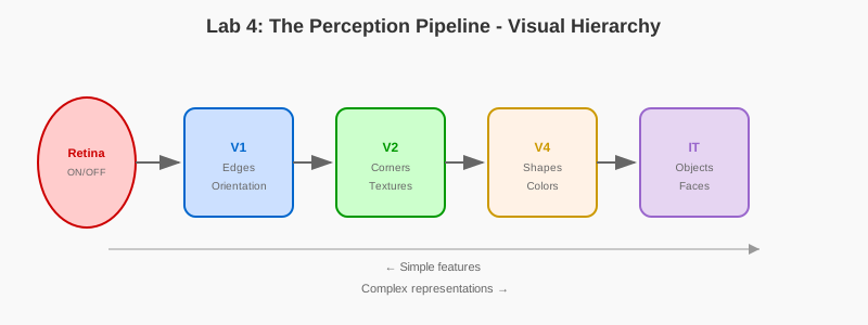
3. Create a simple convolutional neural network mimicking V1-V4-IT pathway
4. Visualize receptive fields and feature maps at different levels
5. Compare biological and artificial visual processing hierarchies

4.2 Prerequisites

• Reading: Chapter 4: The Perception Pipeline
• Libraries: NumPy, Matplotlib, (optional: PyTorch/TensorFlow for CNN)
• Concepts: Convolution, edge detection, hierarchical processing

4.3 Setup

import numpy as np
import matplotlib.pyplot as plt
from scipy import signal, ndimage

np.random.seed(42)

plt.style.use('default')
plt.rcParams['figure.figsize'] = (12, 8)
plt.rcParams['font.size'] = 11

4.4 Part 1: Retinal Processing - Center-Surround

4.4.1 1.1 Center-Surround Receptive Fields

Retinal ganglion cells and LGN neurons have center-surround receptive fields that detect luminance changes.

def create_center_surround_filter(size=15, sigma_center=1.0, sigma_surround=3.0):
    """
    Create Difference-of-Gaussians (DoG) filter.

    This approximates the center-surround receptive field of retinal ganglion cells.
    """
    # Create coordinate grid
    x = np.linspace(-size//2, size//2, size)
    y = np.linspace(-size//2, size//2, size)
    X, Y = np.meshgrid(x, y)

    # Center (excitatory)
    center = np.exp(-(X**2 + Y**2) / (2 * sigma_center**2))
    center = center / np.sum(center)

    # Surround (inhibitory)
    surround = np.exp(-(X**2 + Y**2) / (2 * sigma_surround**2))
    surround = surround / np.sum(surround)

    # Difference of Gaussians
    dog_filter = center - 0.85 * surround

    return dog_filter

## Create ON-center and OFF-center filters
on_center = create_center_surround_filter()
off_center = -on_center

## Visualize
fig, (ax1, ax2) = plt.subplots(1, 2, figsize=(12, 5))

im1 = ax1.imshow(on_center, cmap='RdBu_r', vmin=-0.15, vmax=0.15)
ax1.set_title('ON-Center Receptive Field', fontweight='bold', fontsize=14)
ax1.axis('off')
plt.colorbar(im1, ax=ax1)

im2 = ax2.imshow(off_center, cmap='RdBu_r', vmin=-0.15, vmax=0.15)
ax2.set_title('OFF-Center Receptive Field', fontweight='bold', fontsize=14)
ax2.axis('off')
plt.colorbar(im2, ax=ax2)

plt.tight_layout()
plt.show()

## Test on simple image
test_image = np.zeros((100, 100))
test_image[40:60, 40:60] = 1  # White square

on_response = signal.convolve2d(test_image, on_center, mode='same')
off_response = signal.convolve2d(test_image, off_center, mode='same')

fig, axes = plt.subplots(1, 3, figsize=(15, 5))

axes[0].imshow(test_image, cmap='gray')
axes[0].set_title('Original Image', fontweight='bold')
axes[0].axis('off')

axes[1].imshow(on_response, cmap='RdBu_r')
axes[1].set_title('ON-Center Response\\n(Bright in center)', fontweight='bold')
axes[1].axis('off')

axes[2].imshow(off_response, cmap='RdBu_r')
axes[2].set_title('OFF-Center Response\\n(Dark in center)', fontweight='bold')
axes[2].axis('off')

plt.tight_layout()
plt.show()

4.4.2 1.2 Edge Detection

Center-surround cells are edge detectors - they respond strongly to luminance boundaries.

## Load or create a test image
def create_test_scene():
    \"\"\"Create a simple test scene with edges.\"\"\"
    img = np.ones((200, 200)) * 0.5  # Gray background
    img[50:150, 50:100] = 0.2  # Dark rectangle
    img[50:150, 120:170] = 0.8  # Bright rectangle
    # Add some circles
    Y, X = np.ogrid[:200, :200]
    circle1 = (X - 60)**2 + (Y - 180)**2 < 20**2
    circle2 = (X - 140)**2 + (Y - 180)**2 < 20**2
    img[circle1] = 0.1
    img[circle2] = 0.9
    return img

image = create_test_scene()

## Apply center-surround filtering
dog_response = signal.convolve2d(image, on_center, mode='same')

## Visualize
fig, (ax1, ax2) = plt.subplots(1, 2, figsize=(14, 6))

ax1.imshow(image, cmap='gray')
ax1.set_title('Original Scene', fontweight='bold', fontsize=14)
ax1.axis('off')

ax2.imshow(dog_response, cmap='RdBu_r')
ax2.set_title('Retinal Ganglion Cell Response\\n(Edge Detection)', fontweight='bold', fontsize=14)
ax2.axis('off')

plt.tight_layout()
plt.show()

print(\"Notice: Strong responses at edges and boundaries!\"
      \"\\nThis is the first stage of visual processing.\" )

Exercise 1.1: Create Gabor filters (oriented edge detectors) by multiplying a Gaussian with a sinusoid. These model V1 simple cells.

Exercise 1.2: Apply multiple Gabor filters at different orientations (0°, 45°, 90°, 135°) to an image and visualize the responses.

---

4.5 Part 2: V1 Simple and Complex Cells

4.5.1 2.1 Oriented Edge Detectors (Simple Cells)

V1 simple cells respond to oriented edges at specific positions.

def create_gabor_filter(size=21, wavelength=5, orientation=0, sigma=3):
    \"\"\"
    Create a Gabor filter - models V1 simple cell receptive field.

    Args:
        size: Filter size
        wavelength: Wavelength of sinusoid
        orientation: Orientation in radians
        sigma: Gaussian envelope width
    \"\"\"
    # Create coordinate grid
    x = np.linspace(-size//2, size//2, size)
    y = np.linspace(-size//2, size//2, size)
    X, Y = np.meshgrid(x, y)

    # Rotate coordinates
    X_rot = X * np.cos(orientation) + Y * np.sin(orientation)
    Y_rot = -X * np.sin(orientation) + Y * np.cos(orientation)

    # Gabor filter = Gaussian * sinusoid
    gaussian = np.exp(-(X_rot**2 + Y_rot**2) / (2 * sigma**2))
    sinusoid = np.cos(2 * np.pi * X_rot / wavelength)
    gabor = gaussian * sinusoid

    return gabor

## Create Gabor filters at different orientations
orientations = [0, np.pi/4, np.pi/2, 3*np.pi/4]
orientation_names = ['0° (horizontal)', '45°', '90° (vertical)', '135°']
gabor_filters = [create_gabor_filter(orientation=ori) for ori in orientations]

## Visualize filters
fig, axes = plt.subplots(1, 4, figsize=(16, 4))

for ax, filt, name in zip(axes, gabor_filters, orientation_names):
    im = ax.imshow(filt, cmap='RdBu_r', vmin=-0.3, vmax=0.3)
    ax.set_title(f'Gabor Filter\\n{name}', fontweight='bold')
    ax.axis('off')
    plt.colorbar(im, ax=ax, fraction=0.046)

plt.suptitle('V1 Simple Cell Receptive Fields', fontsize=16, fontweight='bold')
plt.tight_layout()
plt.show()

## Apply to image
responses = [signal.convolve2d(image, filt, mode='same') for filt in gabor_filters]

fig, axes = plt.subplots(2, 2, figsize=(12, 12))
axes = axes.flatten()

for ax, resp, name in zip(axes, responses, orientation_names):
    im = ax.imshow(np.abs(resp), cmap='hot')
    ax.set_title(f'Response to {name}', fontweight='bold')
    ax.axis('off')
    plt.colorbar(im, ax=ax, fraction=0.046)

plt.suptitle('V1 Simple Cell Responses at Different Orientations',
            fontsize=16, fontweight='bold')
plt.tight_layout()
plt.show()

4.5.2 2.2 Position Invariance (Complex Cells)

Complex cells pool over simple cells to achieve position invariance.

def complex_cell_response(image, gabor_filters, pool_size=4):
    \"\"\"
    Model V1 complex cell: pool simple cell responses.

    Complex cells respond to oriented edges but are less position-specific.
    \"\"\"
    responses = []

    for filt in gabor_filters:
        # Simple cell response
        simple_resp = signal.convolve2d(image, filt, mode='same')

        # Energy model: square response
        energy = simple_resp ** 2

        # Pool over local regions (max pooling)
        pooled = ndimage.maximum_filter(energy, size=pool_size)

        responses.append(pooled)

    return responses

## Compute complex cell responses
complex_responses = complex_cell_response(image, gabor_filters, pool_size=8)

fig, axes = plt.subplots(2, 2, figsize=(12, 12))
axes = axes.flatten()

for ax, resp, name in zip(axes, complex_responses, orientation_names):
    im = ax.imshow(resp, cmap='hot')
    ax.set_title(f'Complex Cell Response\\n{name}', fontweight='bold')
    ax.axis('off')
    plt.colorbar(im, ax=ax, fraction=0.046)

plt.suptitle('V1 Complex Cell Responses (Position Invariant)',
            fontsize=16, fontweight='bold')
plt.tight_layout()
plt.show()

Exercise 2.1: Shift the image by a few pixels. How do simple cell responses change? How about complex cell responses?

Exercise 2.2: Implement a "hypercomplex" (end-stopped) cell that responds to edges of specific length.

---

Open In Colab

4.6 Part 3: Hierarchical Feature Learning

4.6.1 3.1 Simple Hierarchical Model

Build a 3-layer hierarchy: edges → corners → shapes

## Layer 1: Edge detectors (already have these)

## Layer 2: Corner/junction detectors
def create_corner_detector(size=15):
    \"\"\"Create filters that detect corners (combinations of oriented edges).\"\"\"
    # L-shaped corner (horizontal + vertical)
    corner = np.zeros((size, size))
    mid = size // 2
    corner[mid, :mid+3] = 1  # Horizontal bar
    corner[:mid+3, mid] = 1  # Vertical bar

    return corner - corner.mean()

## Create corner detectors at different rotations
corner_base = create_corner_detector()
corners = [ndimage.rotate(corner_base, angle, reshape=False)
          for angle in [0, 90, 180, 270]]

## Visualize
fig, axes = plt.subplots(1, 4, figsize=(16, 4))
for ax, corner, angle in zip(axes, corners, [0, 90, 180, 270]):
    im = ax.imshow(corner, cmap='RdBu_r')
    ax.set_title(f'Corner Detector\\n{angle}°', fontweight='bold')
    ax.axis('off')
    plt.colorbar(im, ax=ax, fraction=0.046)

plt.suptitle('Layer 2: Corner/Junction Detectors', fontsize=16, fontweight='bold')
plt.tight_layout()
plt.show()

## Apply corner detectors
corner_responses = [signal.convolve2d(image, corner, mode='same')
                   for corner in corners]

fig, axes = plt.subplots(1, 4, figsize=(16, 4))
for ax, resp, angle in zip(axes, corner_responses, [0, 90, 180, 270]):
    im = ax.imshow(np.abs(resp), cmap='hot')
    ax.set_title(f'Corner Response {angle}°', fontweight='bold')
    ax.axis('off')
    plt.colorbar(im, ax=ax, fraction=0.046)

plt.tight_layout()
plt.show()

4.6.2 3.2 Feature Hierarchy Visualization

def visualize_hierarchy():
    \"\"\"Visualize the hierarchical processing pipeline.\"\"\"

    fig, axes = plt.subplots(3, 4, figsize=(16, 12))

    # Original image
    axes[0, 0].imshow(image, cmap='gray')
    axes[0, 0].set_title('Input Image', fontweight='bold')
    axes[0, 0].axis('off')
    for i in range(1, 4):
        axes[0, i].axis('off')

    # Layer 1: Edge orientation
    for i, (resp, name) in enumerate(zip(responses, orientation_names)):
        if i < 4:
            axes[1, i].imshow(np.abs(resp), cmap='hot')
            axes[1, i].set_title(f'L1: Edges\\n{name}', fontweight='bold')
            axes[1, i].axis('off')

    # Layer 2: Corners
    for i, (resp, angle) in enumerate(zip(corner_responses, [0, 90, 180, 270])):
        axes[2, i].imshow(np.abs(resp), cmap='hot')
        axes[2, i].set_title(f'L2: Corners\\n{angle}°', fontweight='bold')
        axes[2, i].axis('off')

    plt.suptitle('Hierarchical Visual Processing: Retina → V1 → V2',
                fontsize=18, fontweight='bold')
    plt.tight_layout()
    plt.show()

visualize_hierarchy()

Exercise 3.1: Create "blob" detectors (cells that respond to color or texture patches). Where would these fit in the hierarchy?

Exercise 3.2: Implement a simple shape detector (e.g., circle, square) by combining corner and edge information.

---

4.7 Part 4: Connection to CNNs

4.7.1 4.1 Building a Simple Conv Layer

def simple_conv_layer(image, n_filters=8, filter_size=5):
    \"\"\"
    Simple convolutional layer inspired by V1.

    Args:
        image: Input image
        n_filters: Number of filters (like having multiple orientation columns)
        filter_size: Size of receptive fields

    Returns:
        Feature maps
    \"\"\"
    # Create random filters (in real CNN, these are learned)
    filters = []
    for i in range(n_filters):
        orientation = i * np.pi / n_filters
        filt = create_gabor_filter(size=filter_size, orientation=orientation)
        filters.append(filt)

    # Apply filters
    feature_maps = []
    for filt in filters:
        response = signal.convolve2d(image, filt, mode='same')
        # ReLU activation
        response = np.maximum(0, response)
        feature_maps.append(response)

    return np.array(feature_maps), filters

## Apply conv layer
feature_maps, filters = simple_conv_layer(image, n_filters=8)

## Visualize
fig = plt.figure(figsize=(16, 10))

## Show filters
for i in range(8):
    ax = plt.subplot(3, 8, i+1)
    ax.imshow(filters[i], cmap='RdBu_r')
    ax.set_title(f'Filter {i+1}', fontsize=9)
    ax.axis('off')

## Show feature maps
for i in range(8):
    ax = plt.subplot(3, 8, i+9)
    ax.imshow(feature_maps[i], cmap='hot')
    ax.set_title(f'Feature Map {i+1}', fontsize=9)
    ax.axis('off')

## Show max pooled version
for i in range(8):
    ax = plt.subplot(3, 8, i+17)
    pooled = ndimage.maximum_filter(feature_maps[i], size=4)
    ax.imshow(pooled, cmap='hot')
    ax.set_title(f'Pooled {i+1}', fontsize=9)
    ax.axis('off')

plt.suptitle('Convolutional Layer: Filters → Feature Maps → Pooling',
            fontsize=16, fontweight='bold')
plt.tight_layout()
plt.show()

4.7.2 4.2 Comparison Table

import pandas as pd

comparison = {
    'Aspect': [
        'Early features',
        'Hierarchy',
        'Pooling',
        'Learning',
        'Invariances',
        'Receptive field size',
        'Nonlinearity'
    ],
    'Brain (V1-V4-IT)': [
        'Edges, bars (V1)',
        'V1 → V2 → V4 → IT',
        'Complex cells, larger RFs',
        'Hebbian, STDP',
        'Position, scale, rotation',
        'Grows with hierarchy',
        'Spike thresholds, dendrites'
    ],
    'CNN (AlexNet-style)': [
        'Learned edge filters',
        'Conv1 → Conv2 → ... → FC',
        'Max pooling',
        'Backpropagation',
        'Translation (limited)',
        'Grows with depth',
        'ReLU activations'
    ]
}

df = pd.DataFrame(comparison)
print(df.to_string(index=False))

Exercise 4.1: Implement a 2-layer CNN from scratch (no frameworks). Use numpy only. Train it on a simple task like detecting vertical vs. horizontal edges.

Exercise 4.2: Visualize how receptive field size grows with network depth. For a 3-layer CNN with 5x5 filters, what is the effective receptive field at each layer?

---

Open In Colab

4.8 Exercises

4.8.1 Exercise 1: Build a Full Hierarchy

Create a 4-layer processing pipeline: - Layer 1: Oriented edges (8 orientations) - Layer 2: Combinations (corners, T-junctions) - Layer 3: Shape parts (curve, straight segments) - Layer 4: Whole shapes (circle, square, triangle)

Test on simple geometric images.

4.8.2 Exercise 2: Receptive Field Mapping

For a given complex cell in your hierarchy: - Systematically test different input patterns - Map out what it responds to - Characterize its receptive field - Compare to biological recordings

4.8.3 Exercise 3: Invariance Testing

Test different types of invariance: - Translation: Shift object position - Scale: Change object size - Rotation: Rotate object - Illumination: Change brightness

Measure response stability for simple vs. complex cells.

4.8.4 Exercise 4: Attention Mechanism

Implement a simple attention model: - Process entire image through your hierarchy - Use a "saliency map" to weight different locations - Show that attention modulates feature responses - Compare to biological attentional gain modulation

---

4.9 Challenge Problems

4.9.1 Challenge 1: Implement V1 Orientation Columns

Biological V1 is organized into orientation columns: - Create a 2D array of V1 neurons - Assign preferred orientations in a pinwheel pattern - Show that nearby neurons prefer similar orientations - Visualize the orientation preference map

4.9.2 Challenge 2: Sparse Coding

Implement sparse coding for natural image patches: - Extract 1000 image patches (8x8 pixels) - Learn dictionary using sparse coding - Show that learned features resemble Gabor filters - Compare receptive fields to actual V1 neurons

4.9.3 Challenge 3: Build a CNN Visualizer

Create a tool to visualize CNN internals: - Load a pre-trained CNN (e.g., VGG16 first layers) - Visualize filters at each layer - Create activation maximization (find images that maximally activate neurons) - Compare to biological receptive fields

---

Open In Colab

4.10 Discussion Questions

4.10.1 Question 1: Biological Plausibility of CNNs

1. What aspects of CNNs are biologically plausible?
2. What aspects are implausible or unknown in biology?
3. Does biological implausibility matter for AI performance?

4.10.2 Question 2: Hierarchical Processing

1. Why is hierarchical processing beneficial for both brains and AI?
2. Could there be alternative (non-hierarchical) architectures?
3. What evidence supports hierarchy in the brain?

4.10.3 Question 3: Learning vs. Innate Structure

1. How much of visual processing is hardwired vs. learned?
2. Evidence: Newborn animals have oriented V1 cells before visual experience
3. How does this inform AI architecture design?
4. Should we hand-design features or learn everything?

---

4.11 Summary

In this lab, you’ve:

1. Implemented center-surround receptive fields for edge detection
2. Created Gabor filters modeling V1 simple cells
3. Built a hierarchical feature processing pipeline
4. Connected biological vision to CNNs
5. Visualized feature maps and receptive fields at multiple levels

Key Takeaways: - Visual processing is hierarchical: simple features → complex features - Early layers detect local features (edges), later layers detect objects - Pooling provides invariance to position and scale - CNNs directly inspired by biological visual cortex - Both use convolution, hierarchy, and nonlinearity

NeuroAI Connections: - V1 simple cells ↔︎ CNN conv filters - Complex cells ↔︎ Pooling layers - Ventral stream ↔︎ Classification networks - Attention ↔︎ Dynamic routing

Next Steps: Lab 5 explores brain networks and connectivity!

---

Open In Colab

4.12 Part 5: Additional Code from Chapter 4

The following code blocks were migrated from the main book chapter to provide hands-on practice with the concepts.

4.12.1 5.1 Gabor Filters: Complete Implementation with skimage

This implementation includes additional parameters and uses scikit-image for enhanced functionality.

# Run this cell to implement a complete Gabor filter with visualization
import numpy as np
import matplotlib.pyplot as plt
from scipy import ndimage
from skimage import data, color

def create_gabor_filter(size=31, sigma=5.0, theta=0, lambda_val=10.0, gamma=0.5):
    """
    Create a Gabor filter kernel, modeling a V1 simple cell.

    Args:
        size: Filter kernel size (odd number)
        sigma: Standard deviation of Gaussian envelope
        theta: Orientation in degrees (0-180)
        lambda_val: Wavelength of sinusoidal carrier
        gamma: Spatial aspect ratio (ellipticity)

    Returns:
        gabor_kernel: 2D numpy array representing the filter
    """
    theta_rad = np.deg2rad(theta)
    x, y = np.meshgrid(np.arange(-size//2, size//2+1), np.arange(-size//2, size//2+1))

    # Rotate coordinates
    x_theta = x * np.cos(theta_rad) + y * np.sin(theta_rad)
    y_theta = -x * np.sin(theta_rad) + y * np.cos(theta_rad)

    # Gabor function: Gaussian envelope * sinusoidal carrier
    gaussian = np.exp(-(x_theta**2 + (gamma * y_theta)**2) / (2 * sigma**2))
    sinusoid = np.cos(2 * np.pi * x_theta / lambda_val)
    gabor_kernel = gaussian * sinusoid
    return gabor_kernel

# Create and visualize Gabor filters at 8 orientations
fig, axes = plt.subplots(2, 4, figsize=(12, 6))
fig.suptitle('Gabor Filters: Models of V1 Receptive Fields', fontsize=16)
axes = axes.flatten()
orientations = [0, 22.5, 45, 67.5, 90, 112.5, 135, 157.5]

for i, theta in enumerate(orientations):
    gabor = create_gabor_filter(theta=theta)
    axes[i].imshow(gabor, cmap='gray')
    axes[i].set_title(f'{theta}°')
    axes[i].axis('off')

plt.tight_layout(rect=[0, 0, 1, 0.96])
plt.show()

print("Observe: Each filter is tuned to a specific orientation.")
print("V1 neurons show similar selectivity in biological recordings.")

Exercise 5.1: Apply these Gabor filters to a natural image (use skimage.data.camera() or skimage.data.astronaut()). Which orientations respond most strongly to different parts of the image?

4.12.2 5.2 PyTorch CNN Model: V1-V2 Architecture

This implementation shows how modern deep learning frameworks implement the same principles as biological vision.

# Run this cell to build a PyTorch model mimicking V1 simple and complex cells
# Note: Requires PyTorch (pip install torch)

import torch
import torch.nn as nn
import torch.nn.functional as F

class V1_V2_Model(nn.Module):
    """
    A simple CNN model mimicking V1 simple and complex cells.

    Architecture parallels:
    - Conv2d: V1 simple cells (oriented edge detectors)
    - ReLU: Neural firing threshold (nonlinearity)
    - MaxPool2d: V1/V2 complex cells (position invariance)
    """
    def __init__(self):
        super().__init__()
        # V1 Simple Cells: 8 learnable filters (orientation columns)
        self.simple_cells = nn.Conv2d(in_channels=1, out_channels=8, kernel_size=5, padding=2)

        # V2 Complex Cells: Pooling creates spatial invariance
        self.complex_cells = nn.MaxPool2d(kernel_size=2, stride=2)

    def forward(self, x):
        # Pass through simple cells (convolution + ReLU)
        simple_responses = F.relu(self.simple_cells(x))
        # Pass through complex cells (max pooling)
        complex_responses = self.complex_cells(simple_responses)
        return simple_responses, complex_responses

# Create model and test with dummy image
model = V1_V2_Model()

# Create a dummy grayscale image (batch=1, channel=1, height=28, width=28)
dummy_image = torch.randn(1, 1, 28, 28)

# Forward pass
simple_out, complex_out = model(dummy_image)

print(f"Input image shape: {dummy_image.shape}")
print(f"V1-like (simple cell) output shape: {simple_out.shape}")
print(f"V2-like (complex cell) output shape: {complex_out.shape}")
print()
print("Notice:")
print("- Simple cells: 8 feature maps (one per filter)")
print("- Complex cells: Spatial dimensions halved (pooling effect)")

Exercise 5.2: Modify the model to add a second convolutional layer. How does this change the output? What biological region might this second layer correspond to?

4.12.3 5.3 Comparing the Two Implementations

# Run this cell to compare NumPy and PyTorch approaches
import pandas as pd

comparison = {
    'Aspect': [
        'Implementation',
        'Learning',
        'Speed',
        'Flexibility',
        'Best for'
    ],
    'NumPy/SciPy': [
        'Manual filter creation',
        'Fixed filters (no learning)',
        'Fast for small arrays',
        'High (full control)',
        'Understanding concepts'
    ],
    'PyTorch': [
        'nn.Module classes',
        'Learnable parameters',
        'GPU acceleration',
        'High (many layers)',
        'Building real models'
    ]
}

df = pd.DataFrame(comparison)
print(df.to_string(index=False))
print()
print("Both approaches teach the same concepts:")
print("1. Convolutions detect local features")
print("2. Multiple filters create feature maps")
print("3. Pooling builds translation invariance")
print("4. Hierarchies build complex from simple features")

Exercise 5.3: Initialize the PyTorch Conv2d layer with Gabor filters instead of random weights. Compare the feature maps to those from the NumPy implementation.