12 Lab 12: The Building Blocks: Classical Machine Learning Foundations

12.1 Learning Objectives
- Implement basic ML algorithms from scratch
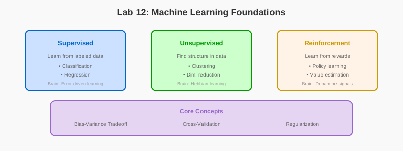
- Compare supervised, unsupervised, and reinforcement learning
- Apply regularization and cross-validation
- Visualize decision boundaries and feature spaces
- Connect ML principles to brain learning mechanisms
12.2 Prerequisites
- Reading: Chapter 12: Machine Learning Foundations
- Libraries: NumPy, Matplotlib, Scikit-learn
- Concepts: Linear models, gradient descent, bias-variance tradeoff
12.3 Setup
import numpy as np
import matplotlib.pyplot as plt
from sklearn.datasets import make_classification, make_moons
from sklearn.model_selection import train_test_split
from sklearn.linear_model import LogisticRegression
from sklearn.tree import DecisionTreeClassifier
from sklearn.metrics import accuracy_score, confusion_matrix

np.random.seed(42)
plt.rcParams['figure.figsize'] = (12, 8)
12.4 Part 1: Linear Classification
## Generate 2D classification data
X, y = make_classification(n_samples=200, n_features=2, n_redundant=0,
                          n_informative=2, n_clusters_per_class=1, random_state=42)

X_train, X_test, y_train, y_test = train_test_split(X, y, test_size=0.3, random_state=42)

## Train logistic regression
clf = LogisticRegression()
clf.fit(X_train, y_train)

## Evaluate
train_acc = accuracy_score(y_train, clf.predict(X_train))
test_acc = accuracy_score(y_test, clf.predict(X_test))

print(f"Train accuracy: {train_acc:.3f}")
print(f"Test accuracy: {test_acc:.3f}")

## Visualize decision boundary
def plot_decision_boundary(clf, X, y, title):
    h = 0.02
    x_min, x_max = X[:, 0].min() - 1, X[:, 0].max() + 1
    y_min, y_max = X[:, 1].min() - 1, X[:, 1].max() + 1
    xx, yy = np.meshgrid(np.arange(x_min, x_max, h),
                        np.arange(y_min, y_max, h))

    Z = clf.predict(np.c_[xx.ravel(), yy.ravel()])
    Z = Z.reshape(xx.shape)

    plt.contourf(xx, yy, Z, alpha=0.3, cmap='RdYlBu')
    plt.scatter(X[:, 0], X[:, 1], c=y, cmap='RdYlBu', edgecolors='black', s=50)
    plt.xlabel('Feature 1')
    plt.ylabel('Feature 2')
    plt.title(title, fontweight='bold')

plt.figure(figsize=(14, 6))

plt.subplot(1, 2, 1)
plot_decision_boundary(clf, X_train, y_train, 'Training Data')

plt.subplot(1, 2, 2)
plot_decision_boundary(clf, X_test, y_test, 'Test Data')

plt.tight_layout()
plt.show()
12.5 Part 2: Bias-Variance Tradeoff
## Compare different model complexities
X_complex, y_complex = make_moons(n_samples=200, noise=0.2, random_state=42)
X_train, X_test, y_train, y_test = train_test_split(X_complex, y_complex,
                                                    test_size=0.3, random_state=42)

depths = [1, 3, 5, 10, 20]
fig, axes = plt.subplots(2, 3, figsize=(16, 10))
axes = axes.flatten()

for ax, depth in zip(axes[:5], depths):
    tree = DecisionTreeClassifier(max_depth=depth, random_state=42)
    tree.fit(X_train, y_train)

    train_acc = accuracy_score(y_train, tree.predict(X_train))
    test_acc = accuracy_score(y_test, tree.predict(X_test))

    plt.sca(ax)
    plot_decision_boundary(tree, X_train, y_train,
                          f'Depth={depth}\\nTrain={train_acc:.2f}, Test={test_acc:.2f}')

axes[5].axis('off')

plt.suptitle('Bias-Variance Tradeoff: Model Complexity', fontsize=16, fontweight='bold')
plt.tight_layout()
plt.show()
12.6 Part 3: K-Means Clustering
from sklearn.cluster import KMeans

## Generate clustered data
n_samples = 300
centers = [[0, 0], [3, 3], [0, 3]]
X_cluster, labels_true = make_classification(n_samples=n_samples, n_features=2,
                                            n_informative=2, n_redundant=0,
                                            n_clusters_per_class=1, n_classes=3,
                                            random_state=42)

## Try different numbers of clusters
fig, axes = plt.subplots(2, 2, figsize=(12, 12))
axes = axes.flatten()

for ax, n_clusters in zip(axes, [2, 3, 4, 5]):
    kmeans = KMeans(n_clusters=n_clusters, random_state=42)
    cluster_labels = kmeans.fit_predict(X_cluster)

    ax.scatter(X_cluster[:, 0], X_cluster[:, 1], c=cluster_labels,
              cmap='viridis', alpha=0.6, edgecolors='black')
    ax.scatter(kmeans.cluster_centers_[:, 0], kmeans.cluster_centers_[:, 1],
              marker='X', s=300, c='red', edgecolors='black', linewidth=2)
    ax.set_title(f'K={n_clusters}, Inertia={kmeans.inertia_:.0f}', fontweight='bold')

plt.suptitle('K-Means Clustering', fontsize=16, fontweight='bold')
plt.tight_layout()
plt.show()
12.7 Part 4: Decision Tree from Scratch
This section implements a decision tree classifier from first principles to build deep intuition for how hierarchical decision-making works. This mirrors the brain’s approach to categorical decisions in the prefrontal cortex.
12.7.1 Understanding the Algorithm
A decision tree makes predictions by asking a series of yes/no questions about features. The key components are:
- Gini Impurity: Measures how “mixed” the classes are at a node. A pure node (all same class) has Gini = 0.
- Best Split: Finds the feature and threshold that most reduces impurity.
- Recursive Growth: Builds the tree by repeatedly splitting until stopping criteria are met.
# Run this cell to implement a Decision Tree from scratch

import numpy as np
import matplotlib.pyplot as plt
from sklearn.datasets import make_classification
from sklearn.model_selection import train_test_split
from sklearn.metrics import accuracy_score

class DecisionTreeNode:
    """
    A node in the decision tree.

    Attributes:
        feature_idx: Index of the feature to split on (None for leaf nodes)
        threshold: Threshold value for the split (None for leaf nodes)
        left: Left child node (values < threshold)
        right: Right child node (values >= threshold)
        value: Predicted class for leaf nodes
    """
    def __init__(self, feature_idx=None, threshold=None, left=None, right=None, *, value=None):
        self.feature_idx = feature_idx
        self.threshold = threshold
        self.left = left
        self.right = right
        self.value = value  # Value if it's a leaf node


class SimpleDecisionTree:
    """
    A simple decision tree classifier built from scratch.

    This implementation uses Gini impurity as the splitting criterion
    and supports a maximum depth parameter to control overfitting.

    Neuroscience Connection:
    Decision trees model hierarchical reasoning in the prefrontal cortex.
    Just as a doctor diagnoses through a series of questions ("fever?" -> "cough?" -> ...),
    this algorithm learns to partition the feature space through binary splits.
    """

    def __init__(self, max_depth=5):
        """
        Initialize the decision tree.

        Args:
            max_depth: Maximum depth of the tree (prevents overfitting)
        """
        self.max_depth = max_depth
        self.root = None

    def fit(self, X, y):
        """
        Build the decision tree from training data.

        Args:
            X: Training features (n_samples, n_features)
            y: Training labels (n_samples,)
        """
        self.root = self._grow_tree(X, y)

    def _gini(self, y):
        """
        Calculate Gini impurity of a node.

        Gini = 1 - sum(p_i^2) where p_i is the proportion of class i

        Interpretation:
        - Gini = 0: Pure node (all same class)
        - Gini = 0.5: Maximum impurity (binary, 50/50 split)

        Args:
            y: Labels at this node

        Returns:
            Gini impurity value (0 to 1 - 1/n_classes)
        """
        m = len(y)
        if m == 0:
            return 0
        _, counts = np.unique(y, return_counts=True)
        p = counts / m
        return 1 - np.sum(p**2)

    def _best_split(self, X, y):
        """
        Find the best feature and threshold to split on.

        For each feature, tries all unique values as thresholds
        and selects the split that minimizes weighted Gini impurity.

        Args:
            X: Features at this node
            y: Labels at this node

        Returns:
            best_idx: Index of best feature to split on
            best_thr: Best threshold value
        """
        m, n = X.shape
        if m <= 1:
            return None, None

        # Gini of the current node (before splitting)
        best_gini = self._gini(y)
        best_idx, best_thr = None, None

        # Try each feature
        for idx in range(n):
            # Try each unique value as a threshold
            thresholds, counts = np.unique(X[:, idx], return_counts=True)
            for thr in thresholds:
                # Split the data
                y_left_mask = X[:, idx] < thr
                y_left, y_right = y[y_left_mask], y[~y_left_mask]

                # Skip if split doesn't divide the data
                if len(y_left) == 0 or len(y_right) == 0:
                    continue

                # Calculate weighted Gini of children
                # Lower is better (more pure)
                gini = (len(y_left) / m) * self._gini(y_left) + \
                       (len(y_right) / m) * self._gini(y_right)

                if gini < best_gini:
                    best_gini = gini
                    best_idx = idx
                    best_thr = thr

        return best_idx, best_thr

    def _grow_tree(self, X, y, depth=0):
        """
        Recursively grow the decision tree.

        Stopping criteria:
        1. Maximum depth reached
        2. Node is pure (all same class)

        Args:
            X: Features at this node
            y: Labels at this node
            depth: Current depth in the tree

        Returns:
            DecisionTreeNode (either internal node or leaf)
        """
        # Stopping criterion: max depth or pure node
        if depth >= self.max_depth or len(np.unique(y)) == 1:
            leaf_value = np.argmax(np.bincount(y))
            return DecisionTreeNode(value=leaf_value)

        # Find the best split
        best_idx, best_thr = self._best_split(X, y)

        # If no split improves purity, make a leaf
        if best_idx is None:
            leaf_value = np.argmax(np.bincount(y))
            return DecisionTreeNode(value=leaf_value)

        # Split the data and recurse
        left_mask = X[:, best_idx] < best_thr
        X_left, y_left = X[left_mask], y[left_mask]
        X_right, y_right = X[~left_mask], y[~left_mask]

        left = self._grow_tree(X_left, y_left, depth + 1)
        right = self._grow_tree(X_right, y_right, depth + 1)

        return DecisionTreeNode(best_idx, best_thr, left, right)

    def predict(self, X):
        """
        Predict class labels for samples.

        Args:
            X: Input features (n_samples, n_features)

        Returns:
            Predicted class labels (n_samples,)
        """
        return np.array([self._traverse_tree(x, self.root) for x in X])

    def _traverse_tree(self, x, node):
        """
        Traverse the tree to make a prediction for a single sample.

        Args:
            x: Single sample features
            node: Current node in the tree

        Returns:
            Predicted class label
        """
        # If leaf node, return the predicted class
        if node.value is not None:
            return node.value

        # Otherwise, traverse left or right based on feature value
        if x[node.feature_idx] < node.threshold:
            return self._traverse_tree(x, node.left)
        return self._traverse_tree(x, node.right)
12.7.2 Training and Visualizing the Decision Tree
# Run this cell to train and visualize the decision tree

# Generate 2D classification data
X, y = make_classification(n_samples=200, n_features=2, n_redundant=0,
                           n_informative=2, random_state=42,
                           n_clusters_per_class=1)

X_train, X_test, y_train, y_test = train_test_split(X, y, test_size=0.2, random_state=42)

# Train our custom decision tree
tree = SimpleDecisionTree(max_depth=3)
tree.fit(X_train, y_train)

# Evaluate performance
train_acc = accuracy_score(y_train, tree.predict(X_train))
test_acc = accuracy_score(y_test, tree.predict(X_test))

print(f"Decision Tree Performance:")
print(f"  Training accuracy: {train_acc:.3f}")
print(f"  Test accuracy: {test_acc:.3f}")

# Visualize decision boundary
xx, yy = np.meshgrid(np.linspace(X[:, 0].min() - 1, X[:, 0].max() + 1, 100),
                     np.linspace(X[:, 1].min() - 1, X[:, 1].max() + 1, 100))
Z = tree.predict(np.c_[xx.ravel(), yy.ravel()]).reshape(xx.shape)

plt.figure(figsize=(10, 7))
plt.contourf(xx, yy, Z, alpha=0.3, cmap='viridis')
plt.scatter(X[:, 0], X[:, 1], c=y, cmap='viridis', edgecolors='k', s=50)
plt.title(f"Decision Tree from Scratch (Test Accuracy: {test_acc:.2f})", fontweight='bold')
plt.xlabel("Feature 1")
plt.ylabel("Feature 2")
plt.colorbar(label='Class')
plt.tight_layout()
plt.show()
12.7.3 Experiment: Effect of Tree Depth
# Run this cell to explore how tree depth affects overfitting

depths = [1, 2, 3, 5, 10]
fig, axes = plt.subplots(1, 5, figsize=(20, 4))

for ax, depth in zip(axes, depths):
    tree = SimpleDecisionTree(max_depth=depth)
    tree.fit(X_train, y_train)

    train_acc = accuracy_score(y_train, tree.predict(X_train))
    test_acc = accuracy_score(y_test, tree.predict(X_test))

    Z = tree.predict(np.c_[xx.ravel(), yy.ravel()]).reshape(xx.shape)

    ax.contourf(xx, yy, Z, alpha=0.3, cmap='viridis')
    ax.scatter(X[:, 0], X[:, 1], c=y, cmap='viridis', edgecolors='k', s=30)
    ax.set_title(f'Depth={depth}\nTrain={train_acc:.2f}, Test={test_acc:.2f}', fontweight='bold')
    ax.set_xlabel('Feature 1')
    ax.set_ylabel('Feature 2')

plt.suptitle('Bias-Variance Tradeoff: Effect of Tree Depth', fontsize=14, fontweight='bold')
plt.tight_layout()
plt.show()

print("\nObservations:")
print("- Depth=1: High bias (underfitting) - decision boundary too simple")
print("- Depth=2-3: Good balance - captures main patterns without overfitting")
print("- Depth=5-10: High variance (overfitting) - complex boundaries that may not generalize")
12.8 Exercises
- Implement gradient descent from scratch
- Build a neural network with NumPy only
- Apply PCA and visualize principal components
- Compare different ML algorithms on same dataset
- Modify the Decision Tree to use entropy/information gain instead of Gini impurity
- Add a min_samples_split parameter to control when nodes can be split
12.9 Summary
Covered ML fundamentals: classification, clustering, bias-variance tradeoff, model selection, and building a decision tree from scratch.