6 Lab 6: Neurostimulation & Plasticity

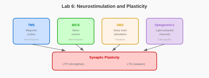
6.1 Learning Objectives
- Model neural responses to electrical stimulation
- Implement basic BCI signal processing and decoding
- Simulate closed-loop neurostimulation systems
- Analyze neural oscillations and their modulation
- Explore therapeutic applications of neurostimulation
6.2 Prerequisites
- Reading: Chapter 6: Neurostimulation
- Libraries: NumPy, Matplotlib, SciPy
- Concepts: Signal processing, filtering, spectral analysis
6.3 Setup
import numpy as np
import matplotlib.pyplot as plt
from scipy import signal
from scipy.fft import fft, fftfreq

np.random.seed(42)
plt.style.use('default')
plt.rcParams['figure.figsize'] = (12, 8)
6.4 Part 1: Neural Oscillations
6.4.1 1.1 Generating Synthetic Neural Signals
def generate_neural_signal(duration=2.0, fs=1000):
    """Generate synthetic LFP signal with multiple frequency bands."""
    t = np.arange(0, duration, 1/fs)

    # Different frequency bands
    delta = 0.5 * np.sin(2 * np.pi * 2 * t)      # 2 Hz
    theta = 0.7 * np.sin(2 * np.pi * 6 * t)      # 6 Hz
    alpha = 0.8 * np.sin(2 * np.pi * 10 * t)     # 10 Hz
    beta = 0.4 * np.sin(2 * np.pi * 20 * t)      # 20 Hz
    gamma = 0.3 * np.sin(2 * np.pi * 40 * t)     # 40 Hz

    # Add noise
    noise = 0.2 * np.random.randn(len(t))

    # Combine
    signal_data = delta + theta + alpha + beta + gamma + noise

    return t, signal_data

## Generate signal
t, lfp_signal = generate_neural_signal()

## Plot time domain
plt.figure(figsize=(14, 8))

plt.subplot(2, 1, 1)
plt.plot(t, lfp_signal, linewidth=1, color='#0066cc')
plt.xlabel('Time (s)', fontsize=12)
plt.ylabel('Amplitude (μV)', fontsize=12)
plt.title('Simulated LFP Signal', fontsize=14, fontweight='bold')
plt.grid(True, alpha=0.3)
plt.xlim(0, 1)  # Show first second

## Plot frequency domain
plt.subplot(2, 1, 2)
freqs = fftfreq(len(lfp_signal), 1/1000)
fft_vals = np.abs(fft(lfp_signal))

positive_freqs = freqs[:len(freqs)//2]
positive_fft = fft_vals[:len(fft_vals)//2]

plt.plot(positive_freqs, positive_fft, linewidth=2, color='#cc0000')
plt.xlabel('Frequency (Hz)', fontsize=12)
plt.ylabel('Power', fontsize=12)
plt.title('Power Spectrum', fontsize=14, fontweight='bold')
plt.grid(True, alpha=0.3)
plt.xlim(0, 50)

plt.tight_layout()
plt.show()
6.4.2 1.2 Band-Pass Filtering
def extract_frequency_band(signal_data, fs, low_freq, high_freq):
    """Extract specific frequency band using bandpass filter."""
    nyquist = fs / 2
    low = low_freq / nyquist
    high = high_freq / nyquist

    b, a = signal.butter(4, [low, high], btype='band')
    filtered = signal.filtfilt(b, a, signal_data)

    return filtered

## Extract different bands
bands = {
    'Delta (1-4 Hz)': (1, 4),
    'Theta (4-8 Hz)': (4, 8),
    'Alpha (8-12 Hz)': (8, 12),
    'Beta (12-30 Hz)': (12, 30),
    'Gamma (30-50 Hz)': (30, 50)
}

fig, axes = plt.subplots(5, 1, figsize=(14, 12))

for ax, (name, (low, high)) in zip(axes, bands.items()):
    filtered = extract_frequency_band(lfp_signal, 1000, low, high)

    ax.plot(t[:1000], filtered[:1000], linewidth=1.5)
    ax.set_ylabel('Amplitude')
    ax.set_title(name, fontweight='bold')
    ax.grid(True, alpha=0.3)

axes[-1].set_xlabel('Time (s)', fontsize=12)
plt.suptitle('Frequency Band Decomposition', fontsize=16, fontweight='bold')
plt.tight_layout()
plt.show()
6.5 Part 2: Electrical Stimulation
6.5.1 2.1 Modeling Stimulation Response
def stimulation_pulse(t, pulse_time, amplitude, width=0.002):
    """Create a stimulation pulse."""
    pulse = np.zeros_like(t)
    mask = (t >= pulse_time) & (t < pulse_time + width)
    pulse[mask] = amplitude
    return pulse

def neural_response_to_stim(stim, tau_rise=0.005, tau_decay=0.05):
    """Model neural response to stimulation (simplified)."""
    # Convolve with alpha function (rise and decay)
    dt = 0.001
    t_kernel = np.arange(0, 0.2, dt)
    kernel = (t_kernel / tau_rise) * np.exp(-t_kernel / tau_decay)
    kernel = kernel / np.max(kernel)

    response = np.convolve(stim, kernel, mode='same')
    return response

## Simulate stimulation train
t = np.arange(0, 2, 0.001)
stim_times = [0.2, 0.4, 0.6, 0.8, 1.0]
stim_signal = np.zeros_like(t)

for stim_t in stim_times:
    stim_signal += stimulation_pulse(t, stim_t, amplitude=1.0)

## Generate response
response = neural_response_to_stim(stim_signal)

## Add background activity
background = 0.1 * np.random.randn(len(t))
total_response = response + background

## Plot
fig, (ax1, ax2) = plt.subplots(2, 1, figsize=(14, 8))

ax1.plot(t, stim_signal, linewidth=2, color='#0066cc')
ax1.set_ylabel('Stimulation\\nAmplitude', fontsize=12)
ax1.set_title('Stimulation Train', fontweight='bold')
ax1.grid(True, alpha=0.3)

ax2.plot(t, total_response, linewidth=1.5, color='#cc0000')
ax2.set_xlabel('Time (s)', fontsize=12)
ax2.set_ylabel('Neural Response\\n(μV)', fontsize=12)
ax2.set_title('Evoked Neural Response', fontweight='bold')
ax2.grid(True, alpha=0.3)

plt.tight_layout()
plt.show()
6.6 Part 3: Brain-Computer Interface Decoding
6.6.1 3.1 Motor Intent Decoding
## Simulate neural activity for different movements
def generate_motor_activity(movement='left', duration=1.0, fs=1000):
    """Generate neural activity patterns for different movements."""
    t = np.arange(0, duration, 1/fs)

    if movement == 'left':
        # Left movement: strong beta suppression, gamma increase
        beta = 0.2 * np.sin(2 * np.pi * 20 * t)
        gamma = 1.5 * np.sin(2 * np.pi * 40 * t)
    elif movement == 'right':
        # Right movement: different pattern
        beta = 1.0 * np.sin(2 * np.pi * 20 * t)
        gamma = 0.3 * np.sin(2 * np.pi * 40 * t)
    else:  # rest
        beta = 0.6 * np.sin(2 * np.pi * 20 * t)
        gamma = 0.6 * np.sin(2 * np.pi * 40 * t)

    noise = 0.3 * np.random.randn(len(t))
    signal_data = beta + gamma + noise

    return t, signal_data

## Generate trials
n_trials = 20
movements = ['left', 'right', 'rest'] * (n_trials // 3)
np.random.shuffle(movements)

features = []
labels = []

for movement in movements:
    _, signal_data = generate_motor_activity(movement)

    # Extract features: beta and gamma power
    beta_filtered = extract_frequency_band(signal_data, 1000, 12, 30)
    gamma_filtered = extract_frequency_band(signal_data, 1000, 30, 50)

    beta_power = np.mean(beta_filtered ** 2)
    gamma_power = np.mean(gamma_filtered ** 2)

    features.append([beta_power, gamma_power])
    labels.append(movement)

features = np.array(features)

## Visualize feature space
plt.figure(figsize=(10, 8))

for movement, color, marker in [('left', 'red', 'o'),
                                ('right', 'blue', 's'),
                                ('rest', 'green', '^')]:
    mask = np.array(labels) == movement
    plt.scatter(features[mask, 0], features[mask, 1],
               c=color, marker=marker, s=150, alpha=0.7,
               label=movement.capitalize(), edgecolors='black', linewidth=1)

plt.xlabel('Beta Power', fontsize=12)
plt.ylabel('Gamma Power', fontsize=12)
plt.title('BCI Feature Space: Neural Signatures of Motor Intent',
         fontsize=14, fontweight='bold')
plt.legend(fontsize=12)
plt.grid(True, alpha=0.3)
plt.tight_layout()
plt.show()
6.7 Part 4: Closed-Loop Stimulation
6.7.1 4.1 Phase-Locked Stimulation
def detect_phase(signal_data, target_phase=0):
    """Detect specific phase of oscillation (simplified)."""
    # Hilbert transform to get instantaneous phase
    analytic_signal = signal.hilbert(signal_data)
    instantaneous_phase = np.angle(analytic_signal)

    return instantaneous_phase

def closed_loop_stimulation(duration=2.0):
    """Simulate closed-loop phase-locked stimulation."""
    fs = 1000
    t = np.arange(0, duration, 1/fs)

    # Generate ongoing theta oscillation
    theta = np.sin(2 * np.pi * 6 * t)
    noise = 0.2 * np.random.randn(len(t))
    neural_signal = theta + noise

    # Extract theta band
    theta_filtered = extract_frequency_band(neural_signal, fs, 4, 8)

    # Detect phase
    phase = detect_phase(theta_filtered)

    # Deliver stimulation at peak (phase = 0)
    stim_signal = np.zeros_like(t)
    threshold = 0.1  # Phase tolerance

    for i in range(100, len(t)-100):  # Avoid edges
        if abs(phase[i]) < threshold and abs(phase[i-1]) > threshold:
            stim_signal[i:i+5] = 0.5

    # Plot
    fig, axes = plt.subplots(3, 1, figsize=(14, 10))

    # Original signal
    axes[0].plot(t, neural_signal, linewidth=1, color='gray', alpha=0.5, label='Raw')
    axes[0].plot(t, theta_filtered, linewidth=2, color='#0066cc', label='Theta filtered')
    axes[0].set_ylabel('Amplitude')
    axes[0].set_title('Neural Signal', fontweight='bold')
    axes[0].legend()
    axes[0].grid(True, alpha=0.3)
    axes[0].set_xlim(0, 1)

    # Phase
    axes[1].plot(t, phase, linewidth=1.5, color='#9966cc')
    axes[1].axhline(y=0, color='red', linestyle='--', label='Target phase')
    axes[1].set_ylabel('Phase (rad)')
    axes[1].set_title('Instantaneous Phase', fontweight='bold')
    axes[1].legend()
    axes[1].grid(True, alpha=0.3)
    axes[1].set_xlim(0, 1)

    # Stimulation
    axes[2].plot(t, stim_signal, linewidth=2, color='#cc0000')
    axes[2].set_xlabel('Time (s)')
    axes[2].set_ylabel('Stim Amplitude')
    axes[2].set_title('Phase-Locked Stimulation Pulses', fontweight='bold')
    axes[2].grid(True, alpha=0.3)
    axes[2].set_xlim(0, 1)

    plt.tight_layout()
    plt.show()

closed_loop_stimulation()
6.8 Exercises
6.8.1 Exercise 1: DBS Parameter Optimization
Simulate deep brain stimulation with varying frequencies (50-200 Hz) and amplitudes. Find optimal parameters.
6.8.2 Exercise 2: P300 BCI
Create a P300 speller simulation - detect event-related potentials for BCI spelling.
6.8.3 Exercise 3: Adaptive Stimulation
Implement an adaptive controller that adjusts stimulation based on measured neural state.
6.8.4 Exercise 4: Multi-Channel Decoding
Extend BCI decoder to use multiple electrode channels and improve classification.
6.9 Challenge Problems
6.9.1 Challenge 1: Real-Time BCI
Implement a simple real-time BCI using streaming data (simulated) with online decoding.
6.9.2 Challenge 2: Seizure Detection and Prevention
Model epileptic activity and design a closed-loop system to detect and abort seizures.
6.9.3 Challenge 3: Optogenetics Simulation
Model optogenetic stimulation with light-gated ion channels and precise temporal control.
6.10 Discussion Questions
6.10.1 Question 1: Invasive vs. Non-Invasive
Compare invasive (implanted electrodes) vs. non-invasive (EEG) approaches for BCI.
6.10.2 Question 2: Ethical Considerations
What ethical issues arise with brain stimulation and BCIs?
6.10.3 Question 3: Therapeutic Applications
How can neurostimulation treat disorders like Parkinson’s, depression, or chronic pain?
6.11 Summary
You’ve explored neural oscillations, electrical stimulation, BCI decoding, and closed-loop systems - the foundations of modern neuroengineering.