7 Lab 7: Information Theory Essentials

7.1 Learning Objectives
By the end of this lab, you will be able to:
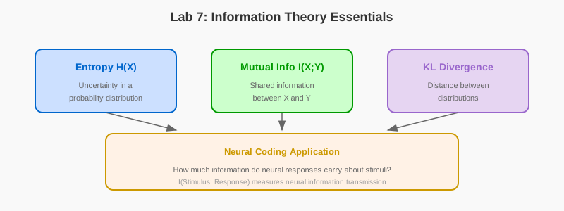
- Calculate and interpret fundamental information-theoretic measures including entropy, mutual information, and KL divergence using Python
- Apply information theory to analyze neural data and quantify information transmission in neural systems
- Implement efficient coding principles including sparse coding and redundancy reduction
- Measure information flow between neural populations and understand population coding strategies
- Connect information-theoretic concepts to both neuroscience applications and AI/ML algorithms
7.2 Prerequisites
- Reading: Chapter 7: Information Theory Essentials
- Libraries: NumPy, Matplotlib, SciPy
- Concepts: Probability distributions, logarithms, correlation
7.3 Setup
import numpy as np
import matplotlib.pyplot as plt
from scipy import stats
from scipy.stats import entropy as scipy_entropy
from sklearn.metrics import mutual_info_score

## Set random seed for reproducibility
np.random.seed(42)

## Set plotting style
plt.style.use('default')
plt.rcParams['figure.figsize'] = (10, 6)
plt.rcParams['font.size'] = 11
7.4 Part 1: Entropy and Surprise
7.4.1 1.1 Understanding Entropy
Entropy measures the uncertainty or “surprise” in a probability distribution. High entropy means high uncertainty (many equally likely outcomes), while low entropy means predictability (one outcome dominates).
Key Formula: \(H(X) = -\sum_{i=1}^{n} p(x_i) \log_2 p(x_i)\)
def entropy(p):
    """Calculate the Shannon entropy of a probability distribution.

    Args:
        p: array of probabilities that sum to 1

    Returns:
        entropy value in bits

    Example:
        >>> entropy(np.array([0.5, 0.5]))  # Fair coin
        1.0
    """
    # Remove zeros to avoid log(0) issues
    p = p[p > 0]
    return -np.sum(p * np.log2(p))

## Example 1: Fair coin toss
p_fair = np.array([0.5, 0.5])
print(f"Entropy of fair coin: {entropy(p_fair):.3f} bits")

## Example 2: Biased coin toss
p_biased = np.array([0.9, 0.1])
print(f"Entropy of biased coin: {entropy(p_biased):.3f} bits")

## Example 3: Fair die
p_die = np.array([1/6] * 6)
print(f"Entropy of fair die: {entropy(p_die):.3f} bits")
Expected Output: - Fair coin: 1.0 bits (maximum entropy for binary variable) - Biased coin: ~0.469 bits (lower because more predictable) - Fair die: ~2.585 bits (need ~3 yes/no questions to identify outcome)
7.4.2 1.2 Visualizing the Binary Entropy Function
The binary entropy function shows how entropy varies with probability for a two-outcome system.
## Visualize entropy for a binary variable as p varies from 0 to 1
p_values = np.linspace(0.001, 0.999, 100)
entropies = [-p*np.log2(p) - (1-p)*np.log2(1-p) for p in p_values]

plt.figure(figsize=(10, 6))
plt.plot(p_values, entropies, linewidth=2, color='#0066cc')
plt.xlabel('Probability of outcome 1', fontsize=12)
plt.ylabel('Entropy (bits)', fontsize=12)
plt.title('Binary Entropy Function', fontsize=14, fontweight='bold')
plt.axvline(x=0.5, color='red', linestyle='--', alpha=0.5, label='Maximum entropy')
plt.axhline(y=1.0, color='gray', linestyle=':', alpha=0.5)
plt.grid(True, alpha=0.3)
plt.legend()
plt.tight_layout()
plt.show()
What to observe: - Entropy is maximized at p=0.5 (complete uncertainty) - Entropy approaches 0 at p=0 or p=1 (complete certainty) - The function is symmetric around p=0.5
7.4.3 1.3 Hands-On: Entropy of Different Distributions
## Compare entropy of different distributions
distributions = {
    'Uniform (4 outcomes)': np.array([0.25, 0.25, 0.25, 0.25]),
    'Slightly biased': np.array([0.4, 0.3, 0.2, 0.1]),
    'Very biased': np.array([0.7, 0.2, 0.08, 0.02]),
    'Nearly deterministic': np.array([0.97, 0.01, 0.01, 0.01])
}

print("Distribution Entropies:")
print("-" * 50)
for name, p in distributions.items():
    H = entropy(p)
    print(f"{name:25s}: {H:.3f} bits")
Exercise 1.1: Create a probability distribution of your choice (must sum to 1) and calculate its entropy. How does it compare to the uniform distribution of the same size?
Exercise 1.2: For a vocabulary of size N, what probability distribution maximizes entropy? What is that maximum entropy value?
7.5 Part 2: Mutual Information
7.5.1 2.1 Understanding Mutual Information
Mutual information measures how much knowing one variable tells you about another. It’s the reduction in uncertainty about X given knowledge of Y.
Key Formula: \(I(X;Y) = H(X) + H(Y) - H(X,Y)\)
def mutual_information(x, y, bins=10):
    """Calculate the mutual information between two continuous variables.

    Args:
        x, y: arrays of observations
        bins: number of bins for discretization

    Returns:
        mutual information value in bits

    Note:
        For continuous variables, we discretize using histograms.
        More bins = better resolution but requires more data.
    """
    # Create joint histogram
    joint_hist, x_edges, y_edges = np.histogram2d(x, y, bins=bins)

    # Normalize to get joint probability
    joint_prob = joint_hist / np.sum(joint_hist)

    # Get marginal probabilities
    x_prob = np.sum(joint_prob, axis=1)
    y_prob = np.sum(joint_prob, axis=0)

    # Calculate mutual information
    mi = 0
    for i in range(bins):
        for j in range(bins):
            if joint_prob[i, j] > 0:
                mi += joint_prob[i, j] * np.log2(
                    joint_prob[i, j] / (x_prob[i] * y_prob[j])
                )

    return mi

## Example: Mutual information between correlated variables
np.random.seed(42)
n = 1000

## Generate correlated data
corr = 0.8
x = np.random.normal(0, 1, n)
y = corr * x + np.sqrt(1 - corr**2) * np.random.normal(0, 1, n)

## Generate independent data for comparison
z = np.random.normal(0, 1, n)

print(f"Mutual information I(X;Y) [correlated]: {mutual_information(x, y):.3f} bits")
print(f"Mutual information I(X;Z) [independent]: {mutual_information(x, z):.3f} bits")
Expected Output: - Correlated variables: ~0.5-0.8 bits - Independent variables: ~0.0-0.1 bits (close to zero)
7.5.2 2.2 MI vs Correlation
## Visualize MI for different correlation values
correlation_values = np.linspace(0, 0.99, 20)
mi_values = []

for c in correlation_values:
    y_corr = c * x + np.sqrt(1 - c**2) * np.random.normal(0, 1, n)
    mi_values.append(mutual_information(x, y_corr, bins=15))

plt.figure(figsize=(10, 6))
plt.plot(correlation_values, mi_values, 'o-', linewidth=2, markersize=6, color='#9966cc')
plt.xlabel('Correlation coefficient', fontsize=12)
plt.ylabel('Mutual information (bits)', fontsize=12)
plt.title('Mutual Information vs. Correlation', fontsize=14, fontweight='bold')
plt.grid(True, alpha=0.3)
plt.tight_layout()
plt.show()
What to observe: - MI increases monotonically with correlation - Even moderate correlation (0.5) gives significant MI - At correlation = 1, variables are perfectly dependent
Exercise 2.1: Create two variables with a non-linear relationship (e.g., y = x²). Calculate both the Pearson correlation and mutual information. What do you observe?
Exercise 2.2: Generate three variables: X, Y (where Y depends on X), and Z (independent). Calculate I(X;Y) and I(X;Z|Y). What does this tell you about conditional independence?
7.6 Part 3: KL Divergence
7.6.1 3.1 Understanding KL Divergence
KL divergence measures how one probability distribution differs from a reference distribution. It’s asymmetric: D_KL(P||Q) ≠ D_KL(Q||P).
Key Formula: \(D_{KL}(P||Q) = \sum_{i} P(i) \log_2 \frac{P(i)}{Q(i)}\)
def kl_divergence(p, q):
    """Calculate the KL divergence between two distributions.

    Args:
        p, q: arrays of probabilities that sum to 1

    Returns:
        KL divergence in bits

    Interpretation:
        D_KL(P||Q) is the "surprise" of using Q when truth is P
    """
    # Filter out zeros to avoid division issues
    mask = (p > 0) & (q > 0)
    p_masked, q_masked = p[mask], q[mask]
    return np.sum(p_masked * np.log2(p_masked / q_masked))

## Example: KL divergence between Gaussians
x = np.linspace(-5, 5, 1000)
p = stats.norm.pdf(x, 0, 1)      # Standard normal (true distribution)
q = stats.norm.pdf(x, 1, 1.5)    # Shifted and wider normal (model)

## Normalize to ensure they sum to 1
p = p / np.sum(p)
q = q / np.sum(q)

print(f"D_KL(P||Q): {kl_divergence(p, q):.3f} bits")
print(f"D_KL(Q||P): {kl_divergence(q, p):.3f} bits")
print(f"\nNote: KL divergence is asymmetric!")

## Visualize
plt.figure(figsize=(10, 6))
x_axis = np.linspace(-5, 5, 1000)
plt.plot(x_axis, p * 1000, label='P ~ N(0,1) [True]', linewidth=2, color='#cc0000')
plt.plot(x_axis, q * 1000, label='Q ~ N(1,1.5) [Model]', linewidth=2,
         color='#0066cc', linestyle='--')
plt.xlabel('x', fontsize=12)
plt.ylabel('Probability density', fontsize=12)
plt.title('KL Divergence Between Distributions', fontsize=14, fontweight='bold')
plt.legend(fontsize=11)
plt.grid(True, alpha=0.3)
plt.tight_layout()
plt.show()
7.6.2 3.2 KL Divergence in Machine Learning
In machine learning, cross-entropy loss is directly related to KL divergence:
Cross-Entropy = H(P,Q) = H(P) + D_KL(P||Q)
When training models, we minimize cross-entropy, which is equivalent to minimizing KL divergence (since H(P) is constant).
Exercise 3.1: Implement cross-entropy loss for a simple classification problem. Show that minimizing cross-entropy is equivalent to minimizing KL divergence between the true and predicted distributions.
Exercise 3.2: Create two probability distributions and calculate both D_KL(P||Q) and D_KL(Q||P). When are they most different? What does this asymmetry mean in practice?
7.7 Part 4: Neural Coding Efficiency
7.7.1 4.1 Measuring Neural Correlations
Efficient neural codes minimize redundancy by decorrelating neural responses.
def calculate_neural_correlations(spike_trains):
    """Calculate pairwise correlations between neural spike trains.

    Args:
        spike_trains: array of shape (n_neurons, n_timepoints)

    Returns:
        correlation matrix of shape (n_neurons, n_neurons)
    """
    n_neurons = spike_trains.shape[0]
    correlations = np.zeros((n_neurons, n_neurons))

    for i in range(n_neurons):
        for j in range(n_neurons):
            correlations[i, j] = np.corrcoef(
                spike_trains[i],
                spike_trains[j]
            )[0, 1]

    return correlations

## Simulate correlated neural data (inefficient code)
np.random.seed(42)
n_neurons = 10
n_timepoints = 1000

## Create correlated spike trains (high redundancy)
base = np.random.rand(n_timepoints)
noise_level = 0.3
spike_trains_redundant = np.array([
    base + noise_level * np.random.randn(n_timepoints)
    for _ in range(n_neurons)
])

## Create decorrelated spike trains (efficient code)
spike_trains_efficient = np.random.randn(n_neurons, n_timepoints)

## Calculate and visualize correlations
corr_redundant = calculate_neural_correlations(spike_trains_redundant)
corr_efficient = calculate_neural_correlations(spike_trains_efficient)

fig, axes = plt.subplots(1, 2, figsize=(12, 5))

im1 = axes[0].imshow(corr_redundant, cmap='coolwarm', vmin=-1, vmax=1)
axes[0].set_title('Redundant Code\n(High Correlations)', fontweight='bold')
axes[0].set_xlabel('Neuron index')
axes[0].set_ylabel('Neuron index')
plt.colorbar(im1, ax=axes[0], label='Correlation')

im2 = axes[1].imshow(corr_efficient, cmap='coolwarm', vmin=-1, vmax=1)
axes[1].set_title('Efficient Code\n(Low Correlations)', fontweight='bold')
axes[1].set_xlabel('Neuron index')
axes[1].set_ylabel('Neuron index')
plt.colorbar(im2, ax=axes[1], label='Correlation')

plt.tight_layout()
plt.show()

## Compare average correlations
avg_corr_redundant = np.mean(np.triu(corr_redundant, k=1))
avg_corr_efficient = np.mean(np.triu(corr_efficient, k=1))

print(f"Average pairwise correlation (redundant): {avg_corr_redundant:.3f}")
print(f"Average pairwise correlation (efficient): {avg_corr_efficient:.3f}")
print(f"\nReduction in redundancy: {(1 - avg_corr_efficient/avg_corr_redundant)*100:.1f}%")
7.7.2 4.2 Sparse Coding
Sparse codes use only a small fraction of neurons at any time, which is energy-efficient and increases storage capacity.
def calculate_sparseness(population_activity):
    """Calculate population sparseness of neural activity.

    Args:
        population_activity: array of shape (n_neurons, n_samples)

    Returns:
        sparseness values for each sample

    Sparseness metric:
        S = (mean(|r|))^2 / mean(r^2)
        S ranges from 1/n (dense) to 1 (maximally sparse)
    """
    n_samples = population_activity.shape[1]
    sparseness = np.zeros(n_samples)

    for i in range(n_samples):
        r = population_activity[:, i]
        if np.sum(r**2) > 0:  # Avoid division by zero
            sparseness[i] = (np.mean(np.abs(r))**2) / np.mean(r**2)

    return sparseness

## Simulate neural populations with different sparseness levels
np.random.seed(42)
n_neurons = 100
n_samples = 10

## Dense coding: many neurons active
dense_pop = np.random.rand(n_neurons, n_samples)

## Sparse coding: few neurons active
sparse_pop = np.zeros((n_neurons, n_samples))
for i in range(n_samples):
    # Only 5% of neurons active
    active_neurons = np.random.choice(n_neurons, size=5, replace=False)
    sparse_pop[active_neurons, i] = np.random.rand(5) * 2

## Calculate sparseness
dense_sparseness = calculate_sparseness(dense_pop)
sparse_sparseness = calculate_sparseness(sparse_pop)

print(f"Average sparseness (dense code): {np.mean(dense_sparseness):.3f}")
print(f"Average sparseness (sparse code): {np.mean(sparse_sparseness):.3f}")

## Visualize
fig, axes = plt.subplots(1, 2, figsize=(12, 5))

im1 = axes[0].imshow(dense_pop, aspect='auto', cmap='viridis')
axes[0].set_title(f'Dense Population\nSparseness: {np.mean(dense_sparseness):.3f}',
                  fontweight='bold')
axes[0].set_xlabel('Sample')
axes[0].set_ylabel('Neuron')
plt.colorbar(im1, ax=axes[0])

im2 = axes[1].imshow(sparse_pop, aspect='auto', cmap='viridis')
axes[1].set_title(f'Sparse Population\nSparseness: {np.mean(sparse_sparseness):.3f}',
                  fontweight='bold')
axes[1].set_xlabel('Sample')
axes[1].set_ylabel('Neuron')
plt.colorbar(im2, ax=axes[1])

plt.tight_layout()
plt.show()
Exercise 4.1: Calculate the total “energy cost” (sum of all neural activity) for dense vs sparse codes representing the same 10 samples. How much energy is saved by sparse coding?
Exercise 4.2: Implement a simple sparse autoencoder using PyTorch or TensorFlow. Train it on image patches and visualize the learned features. Do they resemble the edge detectors found in V1?
7.8 Part 5: Information in Neural Responses
7.8.1 5.1 Spike Train Information
How much information does a neuron’s spike train carry about the stimulus?
def spike_train_information(stimulus, response, bins=10):
    """Calculate mutual information between stimulus and neural response.

    Args:
        stimulus: array of stimulus values
        response: array of neural responses (spike counts)
        bins: number of bins for discretization

    Returns:
        mutual information in bits
    """
    # Discretize continuous variables
    s_bins = np.linspace(min(stimulus), max(stimulus), bins+1)
    r_bins = np.linspace(min(response), max(response), bins+1)

    s_discrete = np.digitize(stimulus, s_bins) - 1
    r_discrete = np.digitize(response, r_bins) - 1

    # Clip to valid range
    s_discrete = np.clip(s_discrete, 0, bins-1)
    r_discrete = np.clip(r_discrete, 0, bins-1)

    # Calculate joint and marginal probabilities
    joint_counts = np.zeros((bins, bins))
    for s, r in zip(s_discrete, r_discrete):
        joint_counts[s, r] += 1

    joint_prob = joint_counts / np.sum(joint_counts)
    s_prob = np.sum(joint_prob, axis=1)
    r_prob = np.sum(joint_prob, axis=0)

    # Calculate mutual information
    mi = 0
    for s in range(bins):
        for r in range(bins):
            if joint_prob[s, r] > 0:
                mi += joint_prob[s, r] * np.log2(
                    joint_prob[s, r] / (s_prob[s] * r_prob[r])
                )

    return mi

## Simulate orientation-tuned neuron
np.random.seed(42)
n_trials = 1000
stimulus = np.random.uniform(-np.pi, np.pi, n_trials)  # Orientations

## Neuron with preferred orientation
preferred_orientation = 0
tuning_width = 0.5

def tuning_curve(stim, preferred, width):
    """Von Mises tuning curve (circular Gaussian)"""
    return np.exp(np.cos(stim - preferred) / width**2) / (2 * np.pi * width**2)

## Generate noisy Poisson spike responses
mean_response = tuning_curve(stimulus, preferred_orientation, tuning_width)
response = np.random.poisson(mean_response * 10)

## Calculate information
info = spike_train_information(stimulus, response, bins=12)
print(f"Stimulus-response information: {info:.3f} bits")

## Visualize tuning curve and responses
fig, axes = plt.subplots(1, 2, figsize=(12, 5))

stim_range = np.linspace(-np.pi, np.pi, 100)
tuning = tuning_curve(stim_range, preferred_orientation, tuning_width)

axes[0].plot(stim_range, tuning * 10, linewidth=2, color='#cc0000')
axes[0].set_xlabel('Stimulus orientation (rad)', fontsize=12)
axes[0].set_ylabel('Mean spike count', fontsize=12)
axes[0].set_title('Neural Tuning Curve', fontweight='bold')
axes[0].grid(True, alpha=0.3)

axes[1].scatter(stimulus, response, alpha=0.3, s=10, color='#0066cc')
axes[1].set_xlabel('Stimulus orientation (rad)', fontsize=12)
axes[1].set_ylabel('Spike count', fontsize=12)
axes[1].set_title(f'Noisy Responses (I = {info:.3f} bits)', fontweight='bold')
axes[1].grid(True, alpha=0.3)

plt.tight_layout()
plt.show()
Exercise 5.1: Modify the tuning width parameter. How does sharper vs broader tuning affect the mutual information? Plot MI vs tuning width.
Exercise 5.2: Compare information from a single neuron vs a population of 10 neurons with different preferred orientations. How does population coding increase information?
7.9 Part 6: Signal, Noise, and Population Coding
7.9.1 6.1 Signal-to-Noise Ratio
def calculate_snr(signal, noise):
    """Calculate signal-to-noise ratio in decibels.

    Args:
        signal: array of signal values
        noise: array of noise values

    Returns:
        SNR in dB
    """
    signal_power = np.mean(signal**2)
    noise_power = np.mean(noise**2)
    if noise_power == 0:
        return np.inf
    snr_db = 10 * np.log10(signal_power / noise_power)
    return snr_db

## Simulate signal with varying noise levels
np.random.seed(42)
t = np.linspace(0, 10, 1000)
signal = np.sin(t) + 0.5 * np.sin(3 * t)
noise_levels = [0.1, 0.5, 1.0, 2.0]

fig, axes = plt.subplots(2, 2, figsize=(12, 8))
axes = axes.flatten()

for i, noise_level in enumerate(noise_levels):
    noise = noise_level * np.random.randn(len(t))
    noisy_signal = signal + noise

    snr = calculate_snr(signal, noise)

    axes[i].plot(t, signal, 'b-', alpha=0.7, linewidth=2, label='Clean signal')
    axes[i].plot(t, noisy_signal, 'r-', alpha=0.5, linewidth=1, label='Noisy signal')
    axes[i].set_title(f'Noise σ = {noise_level}, SNR = {snr:.1f} dB',
                      fontweight='bold')
    axes[i].set_xlabel('Time')
    axes[i].set_ylabel('Amplitude')
    axes[i].legend()
    axes[i].grid(True, alpha=0.3)

plt.tight_layout()
plt.show()
7.9.2 6.2 Population Coding and Correlation
def simulate_population_coding(n_neurons, correlation, n_trials=1000):
    """Simulate a population of neurons with specified correlation structure.

    Args:
        n_neurons: number of neurons in the population
        correlation: correlation coefficient between neurons
        n_trials: number of trials to simulate

    Returns:
        population activity matrix of shape (n_neurons, n_trials)
    """
    # Create correlation matrix
    corr_matrix = np.eye(n_neurons)
    corr_matrix[corr_matrix == 0] = correlation

    # Cholesky decomposition to generate correlated Gaussian data
    L = np.linalg.cholesky(corr_matrix)
    uncorrelated = np.random.randn(n_neurons, n_trials)
    population_activity = np.dot(L, uncorrelated)

    return population_activity

## Simulate populations with different correlation structures
np.random.seed(42)
n_neurons = 20
correlation_levels = [0.0, 0.3, 0.6, 0.9]

fig, axes = plt.subplots(2, 2, figsize=(12, 10))
axes = axes.flatten()

for i, corr in enumerate(correlation_levels):
    population = simulate_population_coding(n_neurons, corr)

    # Calculate correlation matrix
    corr_matrix = np.corrcoef(population)

    # Estimate information capacity using eigenvalue spectrum
    eigenvalues = np.linalg.eigvalsh(corr_matrix)
    # Simple approximation of information capacity
    information_capacity = np.sum(np.log2(1 + np.maximum(eigenvalues, 0)))

    im = axes[i].imshow(corr_matrix, cmap='coolwarm', vmin=-1, vmax=1)
    axes[i].set_title(f'ρ = {corr:.1f}, Info ≈ {information_capacity:.1f} bits',
                      fontweight='bold')
    axes[i].set_xlabel('Neuron index')
    axes[i].set_ylabel('Neuron index')
    plt.colorbar(im, ax=axes[i], label='Correlation', fraction=0.046)

plt.tight_layout()
plt.show()

print("\nKey Observation:")
print("As correlation increases, information capacity decreases.")
print("Independent neurons (ρ=0) carry the most information.")
Exercise 6.1: For a population of N=50 neurons, plot how information capacity scales with correlation (from 0 to 0.95). At what correlation level does capacity drop by 50%?
Exercise 6.2: Implement a simple neural decoder that estimates stimulus orientation from population responses. Compare decoding accuracy for populations with different correlation levels.
7.10 Exercises
7.10.1 Exercise 1: Entropy of Real Data
Load a small dataset (e.g., letter frequencies in English text or pixel intensities in an image) and:
- Calculate the empirical entropy
- Compare it to the theoretical maximum entropy (uniform distribution)
- Calculate the redundancy: R = 1 - H(actual)/H(max)
- Discuss why natural data has redundancy
7.10.2 Exercise 2: Information in Neural Tuning
Simulate a population of 20 neurons with different preferred orientations evenly spaced from -π to π:
- For each neuron, calculate I(stimulus; response)
- Plot information vs. tuning width
- Find the optimal tuning width that maximizes information
- Explain why very narrow or very wide tuning is suboptimal
7.10.3 Exercise 3: Decorrelation Transform
Given a set of correlated neural responses:
- Calculate the correlation matrix
- Perform PCA (eigenvalue decomposition)
- Transform the data to the principal component space
- Show that PCs are decorrelated (verify correlation matrix is diagonal)
- Calculate entropy before and after transformation
7.10.4 Exercise 4: KL Divergence in Learning
Simulate a simple learning process:
- Start with a uniform prior distribution over 10 classes
- Observe 100 samples from a true distribution (non-uniform)
- Update your model distribution to match the data
- Track D_KL(true || model) over iterations
- Plot how KL divergence decreases as the model improves
7.10.5 Exercise 5: Sparse vs Dense Representations
Compare sparse and dense codes for representing 100 random patterns:
- Dense: each pattern activates 50% of neurons
- Sparse: each pattern activates 5% of neurons
- Calculate the average pairwise pattern similarity for both codes
- Estimate the number of distinguishable patterns each code can represent
- Discuss the trade-offs between sparse and dense coding
7.10.6 Exercise 6: Information Bottleneck Visualization
Create a simple 3-layer network (input -> bottleneck -> output):
- Input: 100-dimensional random data with known class labels
- Bottleneck: varying dimensions (2, 5, 10, 20, 50)
- For each bottleneck size, estimate I(X;T) and I(T;Y)
- Plot the information plane: I(X;T) vs I(T;Y)
- Discuss the compression-prediction trade-off
7.10.7 Exercise 7: Mutual Information and Causality
Generate three time series: X(t), Y(t), and Z(t) where: - Y(t) = 0.8*X(t-1) + noise (X causes Y) - Z(t) = independent noise
- Calculate I(X(t); Y(t)) vs I(X(t); Z(t))
- Calculate I(X(t-1); Y(t)) (lagged MI)
- Implement transfer entropy: TE(X→Y) = I(Y(t); X(t-1) | Y(t-1))
- Show that TE detects the causal relationship X→Y but not X→Z
7.11 Challenge Problems
7.11.1 Challenge 1: Efficient Coding of Natural Images
Implement the efficient coding hypothesis for natural images:
- Download a dataset of natural images (e.g., van Hateren database)
- Extract small image patches (e.g., 8x8 pixels)
- Analyze the statistical properties:
- Calculate pixel-pixel correlations
- Measure redundancy
- Compute the power spectrum
- Implement two coding strategies:
- Whitening: Decorrelate using PCA
- ICA: Independent Component Analysis for sparse codes
- Visualize the learned filters/receptive fields
- Compare to actual V1 simple cell receptive fields (Gabor filters)
- Calculate the efficiency: bits per pixel for each coding strategy
Bonus: Show that ICA learns oriented, localized filters similar to V1 neurons.
7.11.2 Challenge 2: Information Bottleneck Theory in Deep Networks
Implement and analyze the Information Bottleneck in a real neural network:
- Train a small neural network on MNIST (e.g., 784-256-128-64-10)
- During training, compute for each layer:
- I(X; T_layer): Information about input
- I(T_layer; Y): Information about output labels
- Track these quantities across training epochs
- Create the “information plane” plot (Shwartz-Ziv & Tishby, 2017)
- Identify two phases:
- Fitting phase: I(T;Y) increases rapidly
- Compression phase: I(X;T) decreases while I(T;Y) plateaus
- Discuss: Do your results support or challenge the Information Bottleneck theory?
Note: This is computationally intensive. Use binning or k-NN methods to estimate MI.
7.11.3 Challenge 3: Predictive Coding Network
Implement a simple predictive coding model:
- Create a two-layer network:
- Top layer: Generates predictions of input
- Bottom layer: Computes prediction errors
- Input: Sequential data (e.g., moving sine wave, video frames)
- Learning rule: Update top layer to minimize prediction error
- Analyze information flow:
- How much information is in the prediction error vs. raw input?
- Calculate I(input; error) over time as the model learns
- Compare to a standard feedforward network
- Discuss: Does predictive coding achieve better compression?
Extensions: - Add multiple layers (hierarchical predictive coding) - Compare to modern architectures (e.g., Vision Transformers with self-attention) - Test on real data (e.g., next-frame prediction in videos)
7.12 Discussion Questions
7.12.1 Question 1: Efficiency vs. Flexibility in Neural Coding
The efficient coding hypothesis suggests brains optimize for the statistics of their environment. However, animals often encounter novel environments.
Trade-off: Discuss the tension between coding efficiency (specialized for expected inputs) and flexibility (handling unexpected inputs). How might the brain balance these competing demands?
Adaptation: What neural mechanisms allow for dynamic adjustment of coding strategies? Consider:
- Synaptic plasticity
- Neuromodulation
- Attention
AI Parallel: How do modern AI systems handle this trade-off?
- Transfer learning
- Domain adaptation
- Few-shot learning
- Meta-learning
Evolution vs. Learning: Which aspects of efficient coding are innate (evolved) vs learned during development? Provide examples from visual system development.
7.12.2 Question 2: Information Theory in Modern AI
Information-theoretic principles are central to many modern AI techniques:
Self-Supervised Learning: Methods like SimCLR maximize mutual information between different views of the same data. Why is this a useful learning objective? How does it relate to the brain’s efficient coding?
Variational Autoencoders: VAEs balance reconstruction accuracy (I(X;Z)) against compression (D_KL(Q||P) for latent distribution). How is this similar to the information bottleneck? What role does the β parameter play?
Attention Mechanisms: Can attention be understood as selective information routing? How might attention increase the mutual information between input and task-relevant features while filtering out irrelevant information?
Adversarial Examples: Deep networks are vulnerable to adversarial perturbations. Can information theory explain this? Consider: Do adversarial examples exploit regions where I(X;Y) is low despite high classification confidence?
7.12.3 Question 3: Limits of Information Theory in Neuroscience
While information theory is powerful, it has limitations:
The Neural Code Problem: Information theory tells us how much information is transmitted but not how it’s encoded. Discuss:
- Rate coding vs temporal coding
- Population codes and their interpretation
- The challenge of cracking the neural code
Computational Constraints: Calculating mutual information requires knowing joint distributions, which is hard for high-dimensional neural data. How do researchers address this? What approximations are commonly used?
Beyond Information Transmission: Neural systems don’t just transmit information—they compute with it. How well does information theory capture:
- Computation and transformation
- Decision-making
- Memory and learning
Meaning and Semantics: Information theory is agnostic to meaning. “Cat” and “Xdj” have the same entropy. How do we incorporate semantics into information-theoretic analyses of brain and AI systems?
7.13 Further Exploration
7.13.1 Recommended Papers
- Shannon (1948): “A Mathematical Theory of Communication” - The foundational paper
- Barlow (1961): “Possible Principles Underlying the Transformation of Sensory Messages” - Efficient coding hypothesis
- Tishby et al. (2000): “The Information Bottleneck Method” - Information bottleneck theory
- Shwartz-Ziv & Tishby (2017): “Opening the Black Box of Deep Neural Networks via Information” - IB in deep learning
7.13.2 Computational Tools
- dit: Python package for discrete information theory
- npeet: Non-parametric entropy estimation
- IDTxl: Information dynamics toolkit (transfer entropy, etc.)
- PyTorch/TensorFlow: For implementing information-based losses
7.13.3 Advanced Topics to Explore
- Transfer entropy and Granger causality
- Information geometry and natural gradients
- Rate-distortion theory
- Integrated Information Theory (IIT) of consciousness
- Quantum information theory
7.14 Summary
In this lab, you’ve learned to:
- Calculate entropy, mutual information, and KL divergence for various distributions
- Analyze neural coding strategies through the lens of information theory
- Quantify redundancy and sparseness in neural populations
- Measure information transmission in simulated neural systems
- Connect information-theoretic principles to both neuroscience and AI
Key takeaways: - Information theory provides a universal language for comparing brains and AI - Efficient coding principles explain many features of neural systems - Modern AI techniques (VAEs, self-supervised learning, attention) are deeply rooted in information theory - Practical computation of information measures requires careful handling of discretization and estimation
Continue exploring these concepts by applying them to real neural data and modern deep learning architectures!