10 Lab 10: Model Fitting and Generalized Linear Models

10.1 Learning Objectives
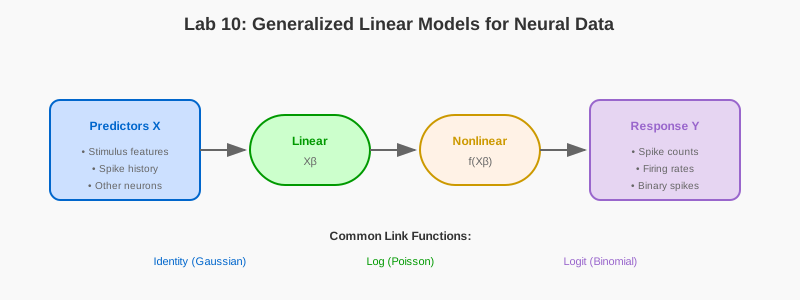
- Fit Generalized Linear Models (GLMs) to neural data
- Compare different link functions and distributions
- Interpret model coefficients and goodness-of-fit
- Build encoding and decoding models
- Cross-validate and avoid overfitting
10.2 Prerequisites
- Reading: Chapter 10: Model Fitting and GLMs
- Libraries: NumPy, Matplotlib, Statsmodels, Scikit-learn
- Concepts: Linear regression, maximum likelihood, model selection
10.3 Setup
Run this cell to import the required libraries and configure the plotting environment:
import numpy as np
import matplotlib.pyplot as plt
from sklearn.model_selection import train_test_split, cross_val_score, KFold
from sklearn.linear_model import Ridge, Lasso, LinearRegression, PoissonRegressor
from sklearn.preprocessing import PolynomialFeatures

np.random.seed(42)
plt.rcParams['figure.figsize'] = (12, 8)
10.4 Part 1: Linear Regression from Scratch
10.4.1 Exercise 1.1: Implementing the Closed-Form Solution
Linear regression is the foundation of many statistical models in neuroscience. In this exercise, you will implement linear regression using the closed-form (analytical) solution to model a neuron’s firing rate as a function of stimulus intensity.
The closed-form solution: \(\boldsymbol{\beta} = (\mathbf{X}^T \mathbf{X})^{-1} \mathbf{X}^T \mathbf{y}\)
Run the following code to implement linear regression from scratch:
def linear_regression_from_scratch():
    """
    Implement linear regression using the closed-form solution.

    Application: Model a neuron's firing rate as a function of stimulus intensity.
    """
    np.random.seed(42)

    # Generate synthetic neural data
    # Scenario: Neuron responds linearly to stimulus with some noise
    n_trials = 200
    stimulus_intensity = np.linspace(0, 10, n_trials)

    # True relationship: firing_rate = 2 + 3 * stimulus + noise
    true_baseline = 2.0
    true_gain = 3.0
    noise = np.random.randn(n_trials) * 1.5

    firing_rate = true_baseline + true_gain * stimulus_intensity + noise

    # Prepare design matrix (add intercept)
    X = np.column_stack([np.ones(n_trials), stimulus_intensity])
    y = firing_rate

    # Closed-form solution: beta = (X^T X)^{-1} X^T y
    beta_hat = np.linalg.inv(X.T @ X) @ X.T @ y

    # Predictions
    y_pred = X @ beta_hat

    # Calculate R-squared
    ss_res = np.sum((y - y_pred) ** 2)
    ss_tot = np.sum((y - y.mean()) ** 2)
    r_squared = 1 - (ss_res / ss_tot)

    # Visualization
    fig, ax = plt.subplots(figsize=(10, 6))
    ax.scatter(stimulus_intensity, firing_rate, alpha=0.5,
               label='Observed data', color='#cc0000')
    ax.plot(stimulus_intensity, y_pred, 'b-', linewidth=2,
            label=f'Fitted model: y = {beta_hat[0]:.2f} + {beta_hat[1]:.2f}x')
    ax.plot(stimulus_intensity, true_baseline + true_gain * stimulus_intensity,
            'g--', linewidth=2, label=f'True model: y = {true_baseline} + {true_gain}x')

    ax.set_xlabel('Stimulus Intensity')
    ax.set_ylabel('Firing Rate (Hz)')
    ax.set_title(f'Linear Regression: Neural Encoding Model (R-squared = {r_squared:.3f})')
    ax.legend()
    ax.grid(alpha=0.3)

    plt.tight_layout()
    plt.show()

    print(f"True parameters: baseline={true_baseline}, gain={true_gain}")
    print(f"Estimated parameters: baseline={beta_hat[0]:.2f}, gain={beta_hat[1]:.2f}")
    print(f"R-squared = {r_squared:.3f}")

    return beta_hat, r_squared

# Run the exercise
linear_regression_from_scratch()
Questions to consider: - How close are the estimated parameters to the true values? - What does the R-squared value tell you about model fit?
10.5 Part 2: Poisson GLM for Spike Trains
10.5.1 Exercise 2.1: Fitting a Poisson GLM
The most common application of GLMs in neuroscience is modeling spike counts using a Poisson distribution. This is appropriate because spike counts are non-negative integers.
Run this code to fit a Poisson GLM to synthetic neural spike data:
def poisson_glm_spike_trains():
    """
    Fit a Poisson GLM to model neural spike counts.

    Scenario: Model how a neuron's spike count depends on stimulus features.
    """
    np.random.seed(42)

    # Generate synthetic spike data
    n_trials = 300

    # Two stimulus features: orientation (0-180 degrees) and contrast (0-1)
    orientation = np.random.rand(n_trials) * 180
    contrast = np.random.rand(n_trials)

    # True relationship (log-linear)
    # log(lambda) = beta0 + beta1 * orientation + beta2 * contrast
    beta_true = np.array([0.5, 0.01, 2.0])

    X = np.column_stack([np.ones(n_trials), orientation, contrast])
    log_rate = X @ beta_true
    rate = np.exp(log_rate)  # Inverse link (exponential)

    # Generate Poisson spike counts
    spike_counts = np.random.poisson(rate)

    # Fit Poisson GLM using scikit-learn
    model = PoissonRegressor(alpha=0, max_iter=1000)
    X_features = X[:, 1:]  # Exclude intercept (model adds it automatically)
    model.fit(X_features, spike_counts)

    # Extract parameters
    beta_hat = np.array([model.intercept_, *model.coef_])

    # Predictions
    rate_pred = np.exp(X @ beta_hat)

    # Visualization
    fig, axes = plt.subplots(1, 2, figsize=(14, 5))

    # Plot 1: Observed vs Predicted spike counts
    axes[0].scatter(rate, spike_counts, alpha=0.4, c='#cc0000', label='Observed')
    max_rate = max(rate.max(), rate_pred.max())
    axes[0].plot([0, max_rate], [0, max_rate], 'k--', label='Perfect prediction')
    axes[0].set_xlabel('True Rate (lambda)')
    axes[0].set_ylabel('Observed Spike Count')
    axes[0].set_title('Poisson GLM: Observed vs True Rate')
    axes[0].legend()
    axes[0].grid(alpha=0.3)

    # Plot 2: Effect of contrast on firing rate
    contrast_range = np.linspace(0, 1, 100)
    orientation_fixed = 90  # Fix orientation at 90 degrees

    X_pred = np.column_stack([
        np.ones(100),
        np.full(100, orientation_fixed),
        contrast_range
    ])
    rate_pred_contrast = np.exp(X_pred @ beta_hat)

    axes[1].plot(contrast_range, rate_pred_contrast, 'b-', linewidth=2,
                 label='Predicted')
    axes[1].set_xlabel('Stimulus Contrast')
    axes[1].set_ylabel('Predicted Firing Rate (Hz)')
    axes[1].set_title(f'Effect of Contrast (orientation={orientation_fixed} degrees)')
    axes[1].grid(alpha=0.3)
    axes[1].legend()

    plt.tight_layout()
    plt.show()

    print("True parameters:", beta_true)
    print("Estimated parameters:", beta_hat)
    print(f"Parameter recovery error: {np.linalg.norm(beta_true - beta_hat):.3f}")

    return beta_hat

# Run the exercise
poisson_glm_spike_trains()
Questions to consider: - Why do we use the log link function for Poisson GLMs? - How does the relationship between contrast and firing rate appear in the plot?
10.6 Part 3: Cross-Validation
10.6.1 Exercise 3.1: Detecting Overfitting with Cross-Validation
Cross-validation is essential for detecting overfitting. This exercise demonstrates how training error can continue to decrease while test error increases with model complexity.
Run this code to see cross-validation in action:
def demonstrate_cross_validation():
    """
    Demonstrate k-fold cross-validation for model evaluation.
    """
    np.random.seed(42)

    # Generate data
    n = 100
    X = np.linspace(0, 10, n).reshape(-1, 1)
    y = 2 + 3 * X.ravel() + 0.5 * X.ravel()**2 + np.random.randn(n) * 5

    # Try different polynomial degrees
    degrees = [1, 2, 3, 5, 10, 15]
    train_scores = []
    cv_scores = []

    for degree in degrees:
        # Create polynomial features
        poly = PolynomialFeatures(degree=degree, include_bias=False)
        X_poly = poly.fit_transform(X)

        # Fit model
        model = Ridge(alpha=0.1)
        model.fit(X_poly, y)

        # Training score
        train_score = model.score(X_poly, y)
        train_scores.append(train_score)

        # 5-fold cross-validation score
        cv_score = cross_val_score(model, X_poly, y, cv=5,
                                   scoring='r2').mean()
        cv_scores.append(cv_score)

    # Plot
    fig, ax = plt.subplots(figsize=(10, 6))
    ax.plot(degrees, train_scores, 'o-', label='Training R-squared',
            color='#0066cc', linewidth=2)
    ax.plot(degrees, cv_scores, 's-', label='Cross-Validation R-squared',
            color='#cc0000', linewidth=2)
    ax.axhline(y=max(cv_scores), color='gray', linestyle='--', alpha=0.5)
    ax.set_xlabel('Polynomial Degree')
    ax.set_ylabel('R-squared Score')
    ax.set_title('Overfitting Detection with Cross-Validation')
    ax.legend()
    ax.grid(alpha=0.3)

    optimal_degree = degrees[np.argmax(cv_scores)]
    print(f"Optimal polynomial degree: {optimal_degree}")
    print(f"Best CV R-squared: {max(cv_scores):.3f}")

    plt.tight_layout()
    plt.show()
    return degrees, train_scores, cv_scores

# Run the exercise
demonstrate_cross_validation()
Questions to consider: - At what polynomial degree does overfitting become apparent? - Why does training R-squared continue to increase while CV R-squared decreases?
10.7 Part 4: Regularization - L1 and L2
10.7.1 Exercise 4.1: Comparing Ridge and Lasso Regularization
Regularization is one of the most effective ways to combat overfitting. This exercise compares L2 (Ridge) and L1 (Lasso) regularization on data with many irrelevant features.
Run this code to compare the two approaches:
def compare_regularization():
    """
    Compare L1 (Lasso) and L2 (Ridge) regularization.
    """
    np.random.seed(42)

    # Generate data with many irrelevant features
    n_samples = 100
    n_features = 50
    n_informative = 5  # Only 5 features are actually relevant

    X = np.random.randn(n_samples, n_features)

    # True coefficients (only first 5 are non-zero)
    beta_true = np.zeros(n_features)
    beta_true[:n_informative] = [3, -2, 4, -1, 2.5]

    y = X @ beta_true + np.random.randn(n_samples) * 0.5

    # Fit models
    ridge = Ridge(alpha=1.0)
    lasso = Lasso(alpha=0.1, max_iter=10000)

    ridge.fit(X, y)
    lasso.fit(X, y)

    # Visualization
    fig, axes = plt.subplots(1, 3, figsize=(15, 5))

    # True coefficients
    axes[0].bar(range(n_features), beta_true, color='gray', alpha=0.7)
    axes[0].set_title('True Coefficients (5 non-zero)')
    axes[0].set_xlabel('Feature Index')
    axes[0].set_ylabel('Coefficient Value')

    # Ridge coefficients
    axes[1].bar(range(n_features), ridge.coef_, color='#0066cc', alpha=0.7)
    axes[1].set_title('Ridge (L2) Regularization (All features shrunk)')
    axes[1].set_xlabel('Feature Index')
    axes[1].set_ylabel('Coefficient Value')

    # Lasso coefficients
    axes[2].bar(range(n_features), lasso.coef_, color='#cc0000', alpha=0.7)
    axes[2].set_title(f'Lasso (L1) Regularization ({np.sum(lasso.coef_ != 0)} non-zero features)')
    axes[2].set_xlabel('Feature Index')
    axes[2].set_ylabel('Coefficient Value')

    for ax in axes:
        ax.axhline(y=0, color='black', linestyle='-', linewidth=0.5)
        ax.grid(alpha=0.3, axis='y')

    plt.tight_layout()
    plt.show()

    print(f"Ridge: {np.sum(ridge.coef_ != 0)} non-zero coefficients")
    print(f"Lasso: {np.sum(lasso.coef_ != 0)} non-zero coefficients")
    print(f"True model: {n_informative} non-zero coefficients")

    return ridge.coef_, lasso.coef_

# Run the exercise
compare_regularization()
Questions to consider: - Which regularization method better recovers the true sparse structure? - When would you prefer Ridge over Lasso, and vice versa?
10.8 Part 5: Model Selection with AIC and BIC
10.8.1 Exercise 5.1: Choosing the Right Model Complexity
Information criteria like AIC and BIC provide a principled way to balance model fit with complexity. This exercise demonstrates how to use them for model selection.
Run this code to compare AIC and BIC for polynomial regression:
def model_selection_demo():
    """
    Demonstrate model selection using AIC and BIC.
    """
    np.random.seed(42)

    # Generate data (true model is quadratic)
    n = 80
    X = np.linspace(0, 10, n).reshape(-1, 1)
    y = 2 + 3*X.ravel() - 0.5*X.ravel()**2 + np.random.randn(n) * 5

    # Try different polynomial degrees
    degrees = range(1, 8)
    aic_scores = []
    bic_scores = []

    for degree in degrees:
        # Fit model
        poly = PolynomialFeatures(degree=degree, include_bias=True)
        X_poly = poly.fit_transform(X)
        model = LinearRegression()
        model.fit(X_poly, y)

        # Calculate residuals
        y_pred = model.predict(X_poly)
        residuals = y - y_pred
        rss = np.sum(residuals**2)

        # Log-likelihood (assuming Gaussian noise)
        n = len(y)
        sigma_sq = rss / n
        log_likelihood = -n/2 * np.log(2 * np.pi * sigma_sq) - rss / (2 * sigma_sq)

        # Number of parameters (including intercept)
        k = degree + 1

        # AIC and BIC
        aic = 2*k - 2*log_likelihood
        bic = k*np.log(n) - 2*log_likelihood

        aic_scores.append(aic)
        bic_scores.append(bic)

    # Plot
    fig, ax = plt.subplots(figsize=(10, 6))
    ax.plot(list(degrees), aic_scores, 'o-', label='AIC',
            color='#0066cc', linewidth=2, markersize=8)
    ax.plot(list(degrees), bic_scores, 's-', label='BIC',
            color='#cc0000', linewidth=2, markersize=8)

    best_aic = list(degrees)[np.argmin(aic_scores)]
    best_bic = list(degrees)[np.argmin(bic_scores)]

    ax.axvline(x=best_aic, color='#0066cc', linestyle='--', alpha=0.5,
               label=f'Best AIC (degree={best_aic})')
    ax.axvline(x=best_bic, color='#cc0000', linestyle='--', alpha=0.5,
               label=f'Best BIC (degree={best_bic})')

    ax.set_xlabel('Polynomial Degree')
    ax.set_ylabel('Information Criterion (lower is better)')
    ax.set_title('Model Selection: AIC vs BIC')
    ax.legend()
    ax.grid(alpha=0.3)

    plt.tight_layout()
    plt.show()

    print(f"Best model by AIC: degree {best_aic}")
    print(f"Best model by BIC: degree {best_bic}")
    print(f"True model: quadratic (degree 2)")

    return aic_scores, bic_scores

# Run the exercise
model_selection_demo()
Questions to consider: - Why does BIC tend to select simpler models than AIC? - Which criterion would you use for predictive vs. explanatory modeling?
10.9 Additional Exercises
- Fit GLMs with different link functions - Try using identity or sqrt links instead of log for Poisson data
- Compare Poisson vs. Negative Binomial - Test on overdispersed data where variance > mean
- Implement regularization (L1/L2) for Poisson GLMs using
PoissonRegressorwith alpha parameter - Build multi-neuron encoding models - Extend the GLM to predict activity from multiple neurons simultaneously
10.10 Summary
In this lab, you have:
- Implemented linear regression from scratch using the closed-form solution
- Fit Poisson GLMs to neural spike count data
- Used cross-validation to detect overfitting
- Compared L1 and L2 regularization techniques
- Applied AIC and BIC for principled model selection
These techniques form the foundation of statistical modeling in computational neuroscience and are essential for building encoding and decoding models of neural activity.