3 Lab 3: The Brain’s GPS: Place Cells, Grid Cells, and Cognitive Maps

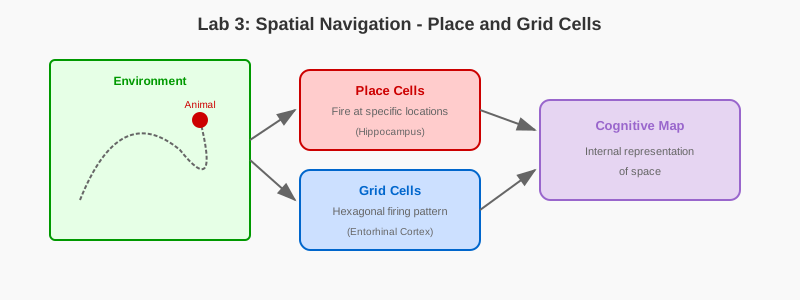
3.1 Learning Objectives
By the end of this lab, you will be able to:
- Simulate place cells and their spatial receptive fields
- Implement grid cell models with hexagonal firing patterns
- Visualize cognitive maps and spatial representations
- Connect neural navigation systems to AI concepts like Graph Neural Networks
- Analyze population coding and path integration mechanisms
3.2 Prerequisites
- Reading: Chapter 3: The Brain’s GPS: Place Cells, Grid Cells, and Cognitive Maps
- Libraries: NumPy, Matplotlib
- Concepts: Spatial representations, population coding, coordinate systems
3.3 Setup
import numpy as np
import matplotlib.pyplot as plt
from matplotlib.patches import Circle, Polygon
from scipy.ndimage import gaussian_filter

## Set random seed
np.random.seed(42)

## Plotting style
plt.style.use('default')
plt.rcParams['figure.figsize'] = (12, 8)
plt.rcParams['font.size'] = 11
3.4 Part 1: Place Cells - The Brain’s Location Markers
3.4.1 1.1 Simulating Place Cells
Place cells fire when an animal is in a specific location - their “place field.”
class PlaceCell:
    \"\"\"Model of a hippocampal place cell.\"\"\"

    def __init__(self, center_x, center_y, field_size=0.3):
        \"\"\"
        Args:
            center_x, center_y: Place field center coordinates (0-1 normalized)
            field_size: Size of place field (larger = wider field)
        \"\"\"
        self.center = np.array([center_x, center_y])
        self.field_size = field_size

    def firing_rate(self, x, y):
        \"\"\"Calculate firing rate at position (x, y).\"\"\"
        distance = np.sqrt((x - self.center[0])**2 + (y - self.center[1])**2)
        # Gaussian firing field
        max_rate = 20  # Hz
        rate = max_rate * np.exp(-(distance**2) / (2 * self.field_size**2))
        return rate

## Create a population of place cells
n_cells = 30
place_cells = []
for i in range(n_cells):
    center_x = np.random.rand()
    center_y = np.random.rand()
    field_size = np.random.uniform(0.15, 0.35)
    place_cells.append(PlaceCell(center_x, center_y, field_size))

## Visualize place fields
fig, axes = plt.subplots(5, 6, figsize=(15, 12))
axes = axes.flatten()

## Create spatial grid
x = np.linspace(0, 1, 50)
y = np.linspace(0, 1, 50)
X, Y = np.meshgrid(x, y)

for idx, cell in enumerate(place_cells):
    # Calculate firing rate across space
    Z = np.zeros_like(X)
    for i in range(len(x)):
        for j in range(len(y)):
            Z[j, i] = cell.firing_rate(X[j, i], Y[j, i])

    # Plot
    im = axes[idx].contourf(X, Y, Z, levels=10, cmap='hot')
    axes[idx].set_title(f'Cell {idx+1}', fontsize=9)
    axes[idx].set_xticks([])
    axes[idx].set_yticks([])
    axes[idx].set_aspect('equal')

plt.suptitle('Place Cell Firing Fields', fontsize=16, fontweight='bold')
plt.tight_layout()
plt.show()
3.4.2 1.2 Population Decoding
Can we decode the animal’s location from the population activity?
def decode_position(place_cells, firing_rates):
    \"\"\"Decode position using population vector.\"\"\"
    # Weighted average of place field centers
    total_rate = np.sum(firing_rates)
    if total_rate == 0:
        return None

    decoded_x = np.sum([cell.center[0] * rate for cell, rate in zip(place_cells, firing_rates)]) / total_rate
    decoded_y = np.sum([cell.center[1] * rate for cell, rate in zip(place_cells, firing_rates)]) / total_rate

    return np.array([decoded_x, decoded_y])

## Simulate animal trajectory
n_steps = 200
trajectory = np.zeros((n_steps, 2))
trajectory[0] = [0.5, 0.5]  # Start at center

## Random walk
for t in range(1, n_steps):
    angle = np.random.rand() * 2 * np.pi
    step = 0.02
    trajectory[t] = trajectory[t-1] + step * np.array([np.cos(angle), np.sin(angle)])
    trajectory[t] = np.clip(trajectory[t], 0, 1)

## Calculate population response and decode position
decoded_positions = []

for pos in trajectory:
    # Get firing rates
    rates = [cell.firing_rate(pos[0], pos[1]) for cell in place_cells]
    # Add Poisson noise
    rates = np.random.poisson(rates)
    # Decode
    decoded = decode_position(place_cells, rates)
    if decoded is not None:
        decoded_positions.append(decoded)
    else:
        decoded_positions.append(pos)

decoded_positions = np.array(decoded_positions)

## Visualize
fig, (ax1, ax2) = plt.subplots(1, 2, figsize=(14, 6))

## True trajectory
ax1.plot(trajectory[:, 0], trajectory[:, 1], 'b-', linewidth=2, alpha=0.7, label='True path')
ax1.scatter(trajectory[0, 0], trajectory[0, 1], s=200, c='green', marker='o',
           edgecolor='black', linewidth=2, label='Start', zorder=5)
ax1.scatter(trajectory[-1, 0], trajectory[-1, 1], s=200, c='red', marker='s',
           edgecolor='black', linewidth=2, label='End', zorder=5)
ax1.set_xlabel('X Position')
ax1.set_ylabel('Y Position')
ax1.set_title('True Trajectory', fontweight='bold')
ax1.legend()
ax1.set_xlim(0, 1)
ax1.set_ylim(0, 1)
ax1.set_aspect('equal')
ax1.grid(True, alpha=0.3)

## Decoded trajectory
ax2.plot(decoded_positions[:, 0], decoded_positions[:, 1], 'r-', linewidth=2, alpha=0.7, label='Decoded path')
ax2.plot(trajectory[:, 0], trajectory[:, 1], 'b--', linewidth=1, alpha=0.4, label='True path')
ax2.scatter(trajectory[0, 0], trajectory[0, 1], s=200, c='green', marker='o',
           edgecolor='black', linewidth=2, label='Start', zorder=5)
ax2.set_xlabel('X Position')
ax2.set_ylabel('Y Position')
ax2.set_title('Decoded Trajectory from Place Cell Activity', fontweight='bold')
ax2.legend()
ax2.set_xlim(0, 1)
ax2.set_ylim(0, 1)
ax2.set_aspect('equal')
ax2.grid(True, alpha=0.3)

plt.tight_layout()
plt.show()

## Calculate decoding error
errors = np.sqrt(np.sum((trajectory - decoded_positions)**2, axis=1))
print(f\"Mean decoding error: {errors.mean():.4f} ± {errors.std():.4f}\")
print(f\"Median decoding error: {np.median(errors):.4f}\")
Exercise 1.1: How does the number of place cells affect decoding accuracy? Try N = [10, 30, 50, 100] and plot error vs. N.
Exercise 1.2: What happens if place fields are very large (field_size = 0.5) vs. very small (field_size = 0.1)? Which gives better decoding?
3.4.3 1.3 Alternative Place Cell Model (from Chapter)
This alternative implementation uses a functional approach to create place cell populations with Gaussian firing fields.
Run this cell to visualize example place cell firing fields using a simplified functional approach.
import numpy as np
import matplotlib.pyplot as plt

def gaussian_2d(x, y, x0, y0, sigma):
    """Generate a 2D Gaussian function."""
    return np.exp(-((x - x0)**2 + (y - y0)**2) / (2 * sigma**2))

def create_place_cell_population(n_cells, env_size, field_sigma):
    """Create a population of place cells."""
    centers = np.random.rand(n_cells, 2) * env_size
    sigmas = np.random.normal(field_sigma, field_sigma * 0.1, n_cells)
    return centers, sigmas

# Simulation
env_size = 10
x = np.linspace(0, env_size, 100)
y = np.linspace(0, env_size, 100)
X, Y = np.meshgrid(x, y)

n_place_cells = 5
centers, sigmas = create_place_cell_population(n_place_cells, env_size, field_sigma=1.0)

# Visualization
fig, axes = plt.subplots(1, n_place_cells, figsize=(15, 3))
fig.suptitle('Example Place Cell Firing Fields', fontsize=16)
for i in range(n_place_cells):
    ax = axes[i]
    place_field = gaussian_2d(X, Y, centers[i, 0], centers[i, 1], sigmas[i])
    im = ax.imshow(place_field, extent=[0, env_size, 0, env_size], origin='lower', cmap='viridis')
    ax.set_title(f'Place Cell {i+1}')
    ax.set_xlabel('X')
    ax.set_ylabel('Y')
plt.tight_layout(rect=[0, 0, 1, 0.95])
plt.show()
Exercise 1.3: Compare this functional approach with the object-oriented PlaceCell class above. What are the advantages and disadvantages of each approach? Which is more extensible for adding complex place cell behaviors?
3.5 Part 2: Grid Cells - Nature’s Coordinate System
3.5.1 2.1 Hexagonal Grid Patterns
Grid cells fire in a beautiful hexagonal lattice pattern across space.
class GridCell:
    \"\"\"Model of an entorhinal cortex grid cell.\"\"\"

    def __init__(self, spacing=0.3, orientation=0, x_offset=0, y_offset=0):
        \"\"\"
        Args:
            spacing: Distance between grid vertices
            orientation: Rotation angle in radians
            x_offset, y_offset: Phase offsets
        \"\"\"
        self.spacing = spacing
        self.orientation = orientation
        self.offset = np.array([x_offset, y_offset])

    def firing_rate(self, x, y):
        \"\"\"Calculate firing rate using 3 cosine gratings (for hexagonal pattern).\"\"\"
        # Rotate coordinates
        cos_o = np.cos(self.orientation)
        sin_o = np.sin(self.orientation)

        x_rot = cos_o * (x - self.offset[0]) - sin_o * (y - self.offset[1])
        y_rot = sin_o * (x - self.offset[0]) + cos_o * (y - self.offset[1])

        # Three gratings at 60° angles create hexagonal pattern
        lambda_ = self.spacing  # Wavelength

        g1 = np.cos(2 * np.pi / lambda_ * x_rot)
        g2 = np.cos(2 * np.pi / lambda_ * (0.5 * x_rot + np.sqrt(3)/2 * y_rot))
        g3 = np.cos(2 * np.pi / lambda_ * (0.5 * x_rot - np.sqrt(3)/2 * y_rot))

        # Sum and threshold
        activation = (g1 + g2 + g3) / 3
        max_rate = 30  # Hz
        rate = max_rate * np.maximum(0, activation + 0.5)  # Shift and rectify

        return rate

## Create grid cells with different scales
grid_spacings = [0.15, 0.25, 0.4, 0.6]
grid_cells = []

for spacing in grid_spacings:
    orientation = np.random.rand() * np.pi / 6  # Small random orientation
    x_offset = np.random.rand() * spacing
    y_offset = np.random.rand() * spacing
    grid_cells.append(GridCell(spacing, orientation, x_offset, y_offset))

## Visualize grid patterns
fig, axes = plt.subplots(2, 2, figsize=(12, 12))
axes = axes.flatten()

x = np.linspace(0, 1.2, 150)
y = np.linspace(0, 1.2, 150)
X, Y = np.meshgrid(x, y)

for idx, cell in enumerate(grid_cells):
    Z = np.zeros_like(X)
    for i in range(len(x)):
        for j in range(len(y)):
            Z[j, i] = cell.firing_rate(X[j, i], Y[j, i])

    im = axes[idx].contourf(X, Y, Z, levels=15, cmap='hot')
    axes[idx].set_title(f'Grid Cell (spacing={grid_spacings[idx]:.2f})', fontweight='bold')
    axes[idx].set_xlabel('X Position')
    axes[idx].set_ylabel('Y Position')
    axes[idx].set_aspect('equal')
    plt.colorbar(im, ax=axes[idx], label='Firing Rate (Hz)')

plt.suptitle('Grid Cell Firing Patterns at Multiple Scales', fontsize=16, fontweight='bold')
plt.tight_layout()
plt.show()
3.5.2 2.2 Multi-Scale Grid Representation
Multiple grid scales provide both precision (fine grid) and range (coarse grid).
def position_from_grids(grid_cells, firing_rates):
    \"\"\"Decode position from grid cell population (simplified).\"\"\"
    # This is a simplified version - actual grid cell decoding is more complex
    # Here we use correlation with expected patterns

    search_x = np.linspace(0, 1, 50)
    search_y = np.linspace(0, 1, 50)

    best_match = 0
    best_pos = None

    for x in search_x:
        for y in search_y:
            expected_rates = [cell.firing_rate(x, y) for cell in grid_cells]
            correlation = np.corrcoef(expected_rates, firing_rates)[0, 1]
            if correlation > best_match:
                best_match = correlation
                best_pos = (x, y)

    return best_pos

## Test position encoding
test_position = (0.5, 0.7)
true_rates = [cell.firing_rate(test_position[0], test_position[1]) for cell in grid_cells]
noisy_rates = [max(0, rate + np.random.randn() * 2) for rate in true_rates]

decoded = position_from_grids(grid_cells, noisy_rates)

print(f\"True position: ({test_position[0]:.3f}, {test_position[1]:.3f})\")
print(f\"Decoded position: ({decoded[0]:.3f}, {decoded[1]:.3f})\")
print(f\"Error: {np.sqrt((test_position[0]-decoded[0])**2 + (test_position[1]-decoded[1])**2):.4f}\")
Exercise 2.1: How many grid scales are needed for accurate position coding? Test with 1, 2, 4, and 6 scales.
Exercise 2.2: What is the optimal ratio between successive grid spacings? Try ratios of 1.4, 1.7, and 2.0.
3.5.3 2.3 Alternative Grid Cell Model (from Chapter)
This implementation uses three interfering plane waves to generate hexagonal patterns, demonstrating the mathematical elegance of grid cell firing.
Run this cell to visualize grid cells with different spacing and orientation parameters.
import numpy as np
import matplotlib.pyplot as plt

def generate_grid_pattern(size, spacing, orientation):
    """Generate a grid cell firing pattern using three interfering plane waves."""
    width, height = size
    grid = np.zeros((height, width))

    # Create 3 vectors for the hexagonal grid (separated by 120 degrees)
    vectors = []
    for i in range(3):
        angle = orientation + i * (2 * np.pi / 3)
        vectors.append(np.array([np.cos(angle), np.sin(angle)]))

    # Generate pattern from interfering plane waves
    for r in range(height):
        for c in range(width):
            pos = np.array([c, r])
            sum_waves = 0
            for v in vectors:
                sum_waves += np.cos(2 * np.pi * np.dot(pos, v) / spacing)
            grid[r, c] = (sum_waves + 3) / 6  # Scale to [0, 1]

    return grid

# Simulation & Visualization
fig, axes = plt.subplots(1, 3, figsize=(15, 5))
fig.suptitle('Grid Cells with Different Spacing and Orientation', fontsize=16)
spacings = [20, 30, 40]
orientations = [0, np.pi/12, np.pi/6]

for i, (spacing, orientation) in enumerate(zip(spacings, orientations)):
    grid_pattern = generate_grid_pattern(size=(100, 100), spacing=spacing, orientation=orientation)
    im = axes[i].imshow(grid_pattern, cmap='magma', origin='lower')
    axes[i].set_title(f'Spacing: {spacing}, Orient: {orientation:.2f}')
    fig.colorbar(im, ax=axes[i], shrink=0.8)

plt.tight_layout(rect=[0, 0, 1, 0.95])
plt.show()
Exercise 2.3: Compare this plane wave interference approach with the cosine grating method in the GridCell class. Do both methods produce equivalent hexagonal patterns? Which is more computationally efficient?
3.6 Part 3: Cognitive Maps and Graph Representations
3.6.1 3.1 Building a Connectivity Graph
Cognitive maps can be represented as graphs where nodes are places and edges are paths.
import networkx as nx

## Create a simple environment graph
G = nx.Graph()

## Add locations (nodes)
locations = ['Home', 'Park', 'Cafe', 'Library', 'Gym', 'Store', 'Office']
G.add_nodes_from(locations)

## Add connections (edges) with distances
edges = [
    ('Home', 'Park', 0.3),
    ('Home', 'Cafe', 0.5),
    ('Park', 'Library', 0.4),
    ('Cafe', 'Store', 0.2),
    ('Cafe', 'Office', 0.6),
    ('Library', 'Gym', 0.3),
    ('Store', 'Office', 0.4),
    ('Gym', 'Store', 0.5),
]

for loc1, loc2, dist in edges:
    G.add_edge(loc1, loc2, weight=dist)

## Visualize the graph
plt.figure(figsize=(10, 8))
pos = nx.spring_layout(G, seed=42)
nx.draw_networkx_nodes(G, pos, node_size=3000, node_color='lightblue',
                       edgecolors='black', linewidths=2)
nx.draw_networkx_labels(G, pos, font_size=12, font_weight='bold')
nx.draw_networkx_edges(G, pos, width=2, alpha=0.6)

## Draw edge labels
edge_labels = nx.get_edge_attributes(G, 'weight')
nx.draw_networkx_edge_labels(G, pos, edge_labels, font_size=10)

plt.title('Cognitive Map as a Graph', fontsize=16, fontweight='bold')
plt.axis('off')
plt.tight_layout()
plt.show()

## Find shortest path
start = 'Home'
goal = 'Office'
path = nx.shortest_path(G, start, goal, weight='weight')
path_length = nx.shortest_path_length(G, start, goal, weight='weight')

print(f\"Shortest path from {start} to {goal}: {' → '.join(path)}\")
print(f\"Total distance: {path_length:.2f}\")
3.6.2 3.2 Path Integration
Animals can track their position by integrating velocity over time (path integration).
class PathIntegrator:
    \"\"\"Simple path integration model.\"\"\"

    def __init__(self, start_pos=[0, 0]):
        self.position = np.array(start_pos, dtype=float)
        self.history = [self.position.copy()]

    def update(self, velocity, dt):
        \"\"\"Update position based on velocity.\"\"\"
        self.position += velocity * dt
        self.history.append(self.position.copy())

    def reset(self, pos):
        \"\"\"Reset to a known position (place recognition).\"\"\"
        self.position = np.array(pos, dtype=float)
        self.history.append(self.position.copy())

## Simulate path integration
integrator = PathIntegrator(start_pos=[0, 0])
dt = 0.1
true_position = np.array([0.0, 0.0])
true_path = [true_position.copy()]

## Random walk with noise
for t in range(200):
    # True velocity
    true_velocity = np.random.randn(2) * 0.5
    true_position += true_velocity * dt
    true_path.append(true_position.copy())

    # Perceived velocity (with noise)
    noise = np.random.randn(2) * 0.05
    perceived_velocity = true_velocity + noise

    integrator.update(perceived_velocity, dt)

    # Occasionally reset to correct accumulated error (like seeing a landmark)
    if t % 50 == 49:
        integrator.reset(true_position)

true_path = np.array(true_path)
estimated_path = np.array(integrator.history)

## Plot
plt.figure(figsize=(10, 8))
plt.plot(true_path[:, 0], true_path[:, 1], 'b-', linewidth=2, label='True path', alpha=0.7)
plt.plot(estimated_path[:, 0], estimated_path[:, 1], 'r--', linewidth=2, label='Path integration', alpha=0.7)
plt.scatter([0], [0], s=200, c='green', marker='o', edgecolor='black',
           linewidth=2, label='Start', zorder=5)

## Mark reset points
reset_points = estimated_path[49::50]
plt.scatter(reset_points[:, 0], reset_points[:, 1], s=150, c='orange', marker='*',
           edgecolor='black', linewidth=1, label='Reset (landmark)', zorder=5)

plt.xlabel('X Position')
plt.ylabel('Y Position')
plt.title('Path Integration with Periodic Correction', fontsize=14, fontweight='bold')
plt.legend()
plt.grid(True, alpha=0.3)
plt.axis('equal')
plt.tight_layout()
plt.show()

## Calculate drift (error accumulation)
errors = np.sqrt(np.sum((true_path - estimated_path)**2, axis=1))
plt.figure(figsize=(10, 5))
plt.plot(errors, linewidth=2, color='#9966cc')
plt.xlabel('Time Step')
plt.ylabel('Position Error')
plt.title('Error Accumulation in Path Integration', fontweight='bold')
plt.axvline(x=49, color='orange', linestyle='--', alpha=0.5, label='Reset')
plt.axvline(x=99, color='orange', linestyle='--', alpha=0.5)
plt.axvline(x=149, color='orange', linestyle='--', alpha=0.5)
plt.axvline(x=199, color='orange', linestyle='--', alpha=0.5)
plt.legend()
plt.grid(True, alpha=0.3)
plt.tight_layout()
plt.show()
Exercise 3.1: How quickly does error accumulate without resets? Remove the reset mechanism and measure drift over time.
Exercise 3.2: Implement a Kalman filter that fuses path integration with place cell observations for better position estimates.
3.6.3 3.3 Alternative Path Integration Model (from Chapter)
This simpler functional implementation demonstrates path integration error accumulation with a circular trajectory.
Run this cell to visualize how errors accumulate during path integration (dead reckoning).
import numpy as np
import matplotlib.pyplot as plt

def simulate_path_integration(velocity_profile, dt, noise_level, n_steps):
    """Simulate path integration with accumulating error."""
    true_path = np.zeros((n_steps + 1, 2))
    estimated_path = np.zeros((n_steps + 1, 2))

    for i in range(n_steps):
        v_true = velocity_profile[i % len(velocity_profile)]
        v_noisy = v_true + np.random.normal(0, noise_level, size=2)

        true_path[i+1] = true_path[i] + v_true * dt
        estimated_path[i+1] = estimated_path[i] + v_noisy * dt

    return true_path, estimated_path

# Simulation
# Define a circular velocity profile
angles = np.linspace(0, 2 * np.pi, 50)
velocities = np.array([np.cos(angles), np.sin(angles)]).T

true_path, estimated_path = simulate_path_integration(
    velocities, dt=0.5, noise_level=0.2, n_steps=100)

# Visualization
plt.figure(figsize=(7, 7))
plt.plot(true_path[:, 0], true_path[:, 1], 'b-', lw=2, label='True Path')
plt.plot(estimated_path[:, 0], estimated_path[:, 1], 'r--', lw=2, label='Estimated Path (Drift)')
plt.scatter(0, 0, c='green', s=150, marker='*', label='Start')
plt.title('Path Integration and Error Accumulation')
plt.xlabel('X Position')
plt.ylabel('Y Position')
plt.legend()
plt.grid(True)
plt.axis('equal')
plt.show()
Exercise 3.3: Compare this circular trajectory simulation with the random walk in the PathIntegrator class. How does the type of movement (circular vs. random) affect error accumulation? Which trajectory is more realistic for animal navigation?
3.7 Exercises
3.7.1 Exercise 1: Remapping
Place cells “remap” when entering a new environment - they create entirely new maps.
Simulate this: - Create place cells for Environment A - Simulate trajectory and neural activity - Switch to Environment B (new place cell centers) - Show that the neural code is completely different
3.7.2 Exercise 2: Head Direction Cells
Implement head direction cells that fire when the animal faces a specific direction: - Create 8 cells for different directions (N, NE, E, SE, S, SW, W, NW) - Simulate a random walk with turning - Decode heading from population activity
3.7.3 Exercise 3: Successor Representation
Implement the successor representation (SR) - a model that predicts future states: - Build a grid world (10x10) - Compute SR matrix using random walks - Show that SR captures spatial relationships - Compare to place cell and grid cell codes
3.7.4 Exercise 4: Graph Neural Network for Spatial Reasoning
Use a simple GNN to solve a navigation problem: - Create a graph of locations - Add features to nodes (reward, obstacles) - Implement message passing to propagate information - Find optimal path using learned node embeddings
3.8 Challenge Problems
3.8.1 Challenge 1: Hippocampal Replay
During rest and sleep, hippocampal neurons “replay” recent trajectories.
Implement this: - Record place cell activity during exploration - Detect and extract replay events (compressed, reactivated sequences) - Show that replayed sequences match real trajectories - Bonus: Show reverse replay (for planning)
3.8.3 Challenge 3: Tolman’s Detour Task
Simulate Tolman’s classic experiment showing cognitive maps: - Train agent on multiple routes in a maze - Block the preferred route - Show that agent takes intelligent detour (not just S-R habit) - Compare: Model-free RL vs. cognitive map
3.9 Discussion Questions
3.9.1 Question 1: Place Cells vs. GPS
- How is the brain’s place cell system similar to GPS? How is it different?
- What advantages does the biological system have?
- Could AI systems benefit from place cell-like representations?
3.9.2 Question 2: Grid Cells and Transformers
Recent work shows connections between grid cells and attention mechanisms.
- How might hexagonal grid patterns relate to multi-head attention?
- Could grid cell codes provide better positional embeddings than sinusoidal encodings?
- What would a “grid cell layer” in a Transformer look like?
3.9.3 Question 3: Cognitive Maps for Abstract Spaces
Place and grid cells don’t just encode physical space - they can represent abstract “concept spaces.”
- How might the same neural machinery support navigation in concept space?
- Give examples: social relationships, musical scales, semantic similarity
- What does this mean for AI architectures that handle abstract reasoning?
3.10 Summary
In this lab, you’ve:
- Implemented place cells and decoded position from population activity
- Modeled grid cells with hexagonal firing patterns
- Explored multi-scale grid representations
- Built graph-based cognitive maps
- Simulated path integration and error correction
Key Takeaways: - The brain uses specialized cells (place, grid, head direction) for spatial navigation - Population coding allows robust, distributed representations - Multi-scale grid codes provide both precision and range - Cognitive maps are graph-like structures enabling flexible planning - Path integration accumulates error and needs periodic correction
NeuroAI Connections: - Graph Neural Networks ↔︎ Cognitive maps - Positional embeddings ↔︎ Grid cells - World models ↔︎ Hippocampal representations - SLAM (robotics) ↔︎ Path integration + place recognition
Next Steps: Lab 4 explores visual perception and the hierarchical processing pipeline!