13 Lab 13: Deep Learning: Training & Optimisation

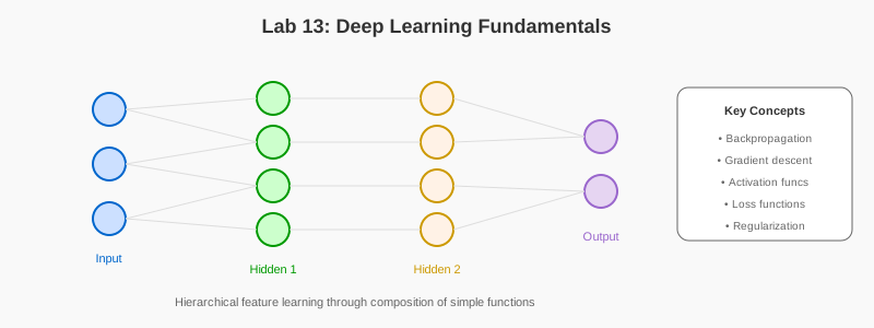
13.1 Learning Objectives
- Build deep neural networks with PyTorch
- Implement optimization algorithms (SGD, Adam)
- Apply regularization techniques
- Train models and visualize learning
- Master deep learning fundamentals
13.2 Prerequisites
- Reading: Chapter 13: Deep Learning
- Libraries: PyTorch, NumPy, Matplotlib
13.3 Setup
import numpy as np
import matplotlib.pyplot as plt
import torch
import torch.nn as nn
import torch.optim as optim

np.random.seed(42)
torch.manual_seed(42)
13.4 Part 1: Building Neural Networks
13.4.1 Exercise 1.1: Simple MLP Implementation
Implement a multilayer perceptron using PyTorch.
class SimpleMLP(nn.Module):
    def __init__(self, input_size, hidden_sizes, output_size):
        """
        A basic multilayer perceptron implementation.

        Args:
            input_size: Number of input features
            hidden_sizes: List of hidden layer sizes
            output_size: Number of output units
        """
        super(SimpleMLP, self).__init__()

        # Create a list to hold all layers
        layers = []

        # Input layer to first hidden layer
        layers.append(nn.Linear(input_size, hidden_sizes[0]))
        layers.append(nn.ReLU())

        # Hidden layers
        for i in range(len(hidden_sizes) - 1):
            layers.append(nn.Linear(hidden_sizes[i], hidden_sizes[i+1]))
            layers.append(nn.ReLU())

        # Final layer
        layers.append(nn.Linear(hidden_sizes[-1], output_size))

        # Combine all layers into a sequential model
        self.model = nn.Sequential(*layers)

    def forward(self, x):
        """Forward pass through the network."""
        return self.model(x)

# Create an example MLP
input_size = 10
hidden_sizes = [128, 64, 32]
output_size = 2
model = SimpleMLP(input_size, hidden_sizes, output_size)

# Display model architecture
print(model)
13.4.2 Exercise 1.2: Activation Functions
Visualize common activation functions used in deep learning.
def plot_activation_functions():
    """Plot common activation functions used in deep learning."""
    # Generate input values
    x = np.linspace(-5, 5, 1000)

    # Calculate activation function outputs
    sigmoid = 1 / (1 + np.exp(-x))
    tanh = np.tanh(x)
    relu = np.maximum(0, x)
    leaky_relu = np.where(x > 0, x, 0.1 * x)
    elu = np.where(x > 0, x, np.exp(x) - 1)

    # Create plot
    plt.figure(figsize=(12, 8))

    plt.plot(x, sigmoid, label='Sigmoid')
    plt.plot(x, tanh, label='Tanh')
    plt.plot(x, relu, label='ReLU')
    plt.plot(x, leaky_relu, label='Leaky ReLU')
    plt.plot(x, elu, label='ELU')

    plt.grid(True)
    plt.legend()
    plt.title('Common Activation Functions')
    plt.xlabel('Input')
    plt.ylabel('Output')
    plt.axhline(y=0, color='k', linestyle='-', alpha=0.3)
    plt.axvline(x=0, color='k', linestyle='-', alpha=0.3)

    plt.tight_layout()
    return plt

plot_activation_functions()
13.4.3 Exercise 1.3: Manual Backpropagation
Demonstrate backpropagation with a simple 2-layer network.
def manual_backpropagation_example():
    """
    Demonstrate backpropagation with a simple 2-layer network.
    """
    # Simple network: Input -> Hidden (2 neurons) -> Output
    # Forward pass
    def sigmoid(x):
        return 1 / (1 + np.exp(-x))

    def sigmoid_derivative(x):
        return x * (1 - x)

    # Network parameters
    input_size = 3
    hidden_size = 2
    output_size = 1

    # Inputs and target
    X = np.array([[0.1, 0.2, 0.3]])
    y_true = np.array([[0.7]])

    # Initialize weights and biases
    np.random.seed(42)
    W1 = np.random.randn(input_size, hidden_size)
    b1 = np.zeros((1, hidden_size))
    W2 = np.random.randn(hidden_size, output_size)
    b2 = np.zeros((1, output_size))

    # Forward pass
    hidden_input = np.dot(X, W1) + b1
    hidden_output = sigmoid(hidden_input)
    final_input = np.dot(hidden_output, W2) + b2
    y_pred = sigmoid(final_input)

    # Calculate loss
    loss = 0.5 * np.sum((y_pred - y_true) ** 2)

    # Backpropagation
    # Output layer error
    output_error = y_pred - y_true
    output_delta = output_error * sigmoid_derivative(y_pred)

    # Hidden layer error
    hidden_error = np.dot(output_delta, W2.T)
    hidden_delta = hidden_error * sigmoid_derivative(hidden_output)

    # Update weights and biases
    learning_rate = 0.1
    W2 -= learning_rate * np.dot(hidden_output.T, output_delta)
    b2 -= learning_rate * np.sum(output_delta, axis=0, keepdims=True)
    W1 -= learning_rate * np.dot(X.T, hidden_delta)
    b1 -= learning_rate * np.sum(hidden_delta, axis=0, keepdims=True)

    return {
        'Initial prediction': y_pred[0][0],
        'Target': y_true[0][0],
        'Loss': loss,
        'Output delta': output_delta[0][0],
        'Hidden delta': hidden_delta[0]
    }

manual_backpropagation_example()
13.4.4 Exercise 1.4: Gradient Problems
Visualize vanishing/exploding gradient problems in deep networks.
def demonstrate_gradient_problems():
    """
    Visualize vanishing/exploding gradient problems in deep networks.
    """
    depths = list(range(1, 21))

    # Vanishing gradient with sigmoid
    vanishing_grads = [0.25 ** d for d in depths]

    # Exploding gradient with poor initialization
    exploding_grads = [1.5 ** d for d in depths]

    # Plot
    plt.figure(figsize=(10, 6))
    plt.semilogy(depths, vanishing_grads, 'b-', label='Vanishing Gradient (sigmoid)')
    plt.semilogy(depths, exploding_grads, 'r-', label='Exploding Gradient (poor init)')
    plt.semilogy(depths, [0.1] * len(depths), 'g--', label='Stable Gradient (with techniques)')

    plt.xlabel('Network Depth (layers)')
    plt.ylabel('Gradient Magnitude (log scale)')
    plt.title('Vanishing and Exploding Gradients in Deep Networks')
    plt.legend()
    plt.grid(True)

    plt.tight_layout()
    return plt

demonstrate_gradient_problems()
13.5 Part 2: Optimization Algorithms
13.5.1 Exercise 2.1: SGD Implementation
Implement basic SGD with mini-batch training.
def sgd_optimizer_example():
    """Implement basic SGD and variants."""
    # Generate dummy data
    np.random.seed(42)
    X = np.random.randn(1000, 10)
    w_true = np.random.randn(10, 1)
    y = X @ w_true + 0.1 * np.random.randn(1000, 1)

    # Initialize parameters
    w = np.zeros((10, 1))

    # SGD parameters
    learning_rate = 0.01
    batch_size = 32
    epochs = 100

    # Training loop
    losses = []
    for epoch in range(epochs):
        # Shuffle data
        indices = np.random.permutation(len(X))
        X_shuffled = X[indices]
        y_shuffled = y[indices]

        epoch_losses = []
        # Process mini-batches
        for i in range(0, len(X), batch_size):
            X_batch = X_shuffled[i:i+batch_size]
            y_batch = y_shuffled[i:i+batch_size]

            # Forward pass
            y_pred = X_batch @ w
            loss = np.mean((y_pred - y_batch) ** 2)
            epoch_losses.append(loss)

            # Backward pass (compute gradient)
            grad = 2 * X_batch.T @ (y_pred - y_batch) / batch_size

            # Update parameters
            w = w - learning_rate * grad

        losses.append(np.mean(epoch_losses))

    return {
        'weights': w,
        'true_weights': w_true,
        'final_loss': losses[-1],
        'loss_history': losses
    }

result = sgd_optimizer_example()
print(f"Final loss: {result['final_loss']:.4f}")
13.5.2 Exercise 2.2: Optimizer Comparison
Compare convergence speed of different optimizers.
def compare_optimizers():
    """Compare convergence speed of different optimizers."""
    import torch
    import torch.nn as nn
    import torch.optim as optim

    # Define a simple problem
    X = torch.randn(1000, 20)
    y = torch.randn(1000, 1)

    # Define model
    model = nn.Sequential(
        nn.Linear(20, 64),
        nn.ReLU(),
        nn.Linear(64, 1)
    )

    # Loss function
    criterion = nn.MSELoss()

    # Define optimizers
    optimizers = {
        'SGD': optim.SGD(model.parameters(), lr=0.01),
        'SGD+Momentum': optim.SGD(model.parameters(), lr=0.01, momentum=0.9),
        'Adam': optim.Adam(model.parameters(), lr=0.01),
        'RMSprop': optim.RMSprop(model.parameters(), lr=0.01),
        'AdamW': optim.AdamW(model.parameters(), lr=0.01, weight_decay=1e-4)
    }

    # Training loops
    results = {}

    for name, optimizer in optimizers.items():
        # Reset model
        model = nn.Sequential(
            nn.Linear(20, 64),
            nn.ReLU(),
            nn.Linear(64, 1)
        )

        # Train
        losses = []
        for epoch in range(100):
            optimizer.zero_grad()
            outputs = model(X)
            loss = criterion(outputs, y)
            losses.append(loss.item())
            loss.backward()
            optimizer.step()

        results[name] = losses

    # Plot
    plt.figure(figsize=(10, 6))
    for name, loss_history in results.items():
        plt.plot(loss_history, label=name)

    plt.xlabel('Epoch')
    plt.ylabel('Loss')
    plt.title('Optimizer Convergence Comparison')
    plt.legend()
    plt.yscale('log')
    plt.grid(True)

    plt.tight_layout()
    return plt

compare_optimizers()
13.5.3 Exercise 2.3: Learning Rate Schedules
Visualize common learning rate schedules.
def learning_rate_schedules():
    """Visualize common learning rate schedules."""
    epochs = np.arange(1, 101)

    # Constant
    constant_lr = [0.1] * 100

    # Step decay
    step_lr = [0.1 * (0.1 ** (e // 30)) for e in epochs]

    # Exponential decay
    exp_lr = [0.1 * np.exp(-0.03 * e) for e in epochs]

    # Cosine annealing
    cosine_lr = [0.1 * (1 + np.cos(np.pi * e / 100)) / 2 for e in epochs]

    # Linear warmup + cosine decay
    warmup = 10
    warmup_cosine_lr = []
    for e in epochs:
        if e <= warmup:
            lr = 0.1 * e / warmup
        else:
            lr = 0.1 * (1 + np.cos(np.pi * (e - warmup) / (100 - warmup))) / 2
        warmup_cosine_lr.append(lr)

    # Plot
    plt.figure(figsize=(10, 6))
    plt.plot(epochs, constant_lr, label='Constant')
    plt.plot(epochs, step_lr, label='Step Decay')
    plt.plot(epochs, exp_lr, label='Exponential Decay')
    plt.plot(epochs, cosine_lr, label='Cosine Annealing')
    plt.plot(epochs, warmup_cosine_lr, label='Warmup + Cosine')

    plt.xlabel('Epoch')
    plt.ylabel('Learning Rate')
    plt.title('Learning Rate Schedules')
    plt.legend()
    plt.yscale('log')
    plt.grid(True)

    plt.tight_layout()
    return plt

learning_rate_schedules()
13.5.4 Exercise 2.4: Second-Order Methods
Compare first and second-order optimization methods.
def second_order_methods():
    """Compare first and second-order optimization methods."""
    # Generate a 2D quadratic function with conditioning issues
    def f(x, y):
        return 0.01 * x**2 + 5 * y**2

    def grad_f(x, y):
        return np.array([0.02 * x, 10 * y])

    def hessian_f(x, y):
        return np.array([[0.02, 0], [0, 10]])

    # Starting point
    x0, y0 = 10.0, 2.0

    # SGD trajectory
    sgd_path = [(x0, y0)]
    x, y = x0, y0
    lr = 0.1
    for _ in range(20):
        g = grad_f(x, y)
        x -= lr * g[0]
        y -= lr * g[1]
        sgd_path.append((x, y))

    # Newton's method trajectory
    newton_path = [(x0, y0)]
    x, y = x0, y0
    for _ in range(5):  # Usually converges in fewer steps
        g = grad_f(x, y)
        H = hessian_f(x, y)
        H_inv = np.linalg.inv(H)
        update = H_inv @ g
        x -= update[0]
        y -= update[1]
        newton_path.append((x, y))

    # Plot
    x_range = np.linspace(-10, 10, 100)
    y_range = np.linspace(-2, 2, 100)
    X, Y = np.meshgrid(x_range, y_range)
    Z = f(X, Y)

    plt.figure(figsize=(10, 8))

    # Contour plot
    plt.contour(X, Y, Z, 20, cmap='viridis', alpha=0.6)

    # Plot paths
    sgd_path = np.array(sgd_path)
    newton_path = np.array(newton_path)

    plt.plot(sgd_path[:, 0], sgd_path[:, 1], 'r.-', label='SGD', linewidth=2, markersize=8)
    plt.plot(newton_path[:, 0], newton_path[:, 1], 'b.-', label="Newton's Method", linewidth=2, markersize=8)

    plt.xlabel('x')
    plt.ylabel('y')
    plt.title("Comparison of First-Order vs. Second-Order Methods")
    plt.legend()
    plt.grid(True)

    plt.tight_layout()
    return plt

second_order_methods()
13.6 Part 3: Regularization Techniques
13.6.1 Exercise 3.1: Dropout and Batch Normalization
Implement and visualize dropout and batch normalization effects.
def dropout_example():
    """Implement and visualize dropout."""
    import torch
    import torch.nn as nn

    # Define a model with dropout
    class MLPWithDropout(nn.Module):
        def __init__(self, dropout_rate=0.5):
            super().__init__()
            self.fc1 = nn.Linear(784, 256)
            self.dropout1 = nn.Dropout(dropout_rate)
            self.fc2 = nn.Linear(256, 128)
            self.dropout2 = nn.Dropout(dropout_rate)
            self.fc3 = nn.Linear(128, 10)

        def forward(self, x):
            x = torch.relu(self.fc1(x))
            x = self.dropout1(x)
            x = torch.relu(self.fc2(x))
            x = self.dropout2(x)
            x = self.fc3(x)
            return x

    # Create a toy example for visualization
    model = MLPWithDropout(dropout_rate=0.5)

    # Generate random activations for demonstration
    activations = torch.rand(1, 256)

    # Apply dropout with different rates
    dropout_rates = [0.0, 0.3, 0.5, 0.7]
    results = []

    for rate in dropout_rates:
        dropout = nn.Dropout(rate)
        dropout.train()
        dropped_activations = dropout(activations)
        results.append((rate, dropped_activations[0].detach().numpy()))

    # Visualize
    fig, axes = plt.subplots(len(dropout_rates), 1, figsize=(10, 8))

    for i, (rate, acts) in enumerate(results):
        axes[i].bar(range(50), acts[:50], alpha=0.7)
        axes[i].set_title(f'Dropout Rate: {rate}')
        axes[i].set_ylim(0, 1.5)
        axes[i].grid(True, alpha=0.3)

    plt.tight_layout()
    return fig

dropout_example()
def batch_norm_example():
"""Demonstrate batch normalization effect."""
import torch
import torch.nn as nn
# Create random activations
np.random.seed(42)
activations = np.random.randn(100, 32) * 10 + 5
# Apply batch normalization
bn = nn.BatchNorm1d(32)
normalized = bn(torch.tensor(activations, dtype=torch.float32))
normalized = normalized.detach().numpy()
# Visualize
fig, axes = plt.subplots(2, 1, figsize=(10, 8))
for i in range(5):
axes[0].hist(activations[:, i], alpha=0.3, bins=20, label=f'Feature {i+1}')
axes[0].set_title('Before Batch Normalization')
axes[0].grid(True, alpha=0.3)
axes[0].legend()
for i in range(5):
axes[1].hist(normalized[:, i], alpha=0.3, bins=20, label=f'Feature {i+1}')
axes[1].set_title('After Batch Normalization')
axes[1].grid(True, alpha=0.3)
axes[1].legend()
plt.tight_layout()
return fig
batch_norm_example()13.6.2 Exercise 3.2: Weight Decay and Early Stopping
Visualize weight decay effects and early stopping.
def weight_decay_visualization():
    """Visualize the effect of weight decay on model complexity."""
    from sklearn.linear_model import Ridge
    from sklearn.preprocessing import PolynomialFeatures
    from sklearn.pipeline import make_pipeline

    # Generate synthetic data
    np.random.seed(42)
    X = np.sort(np.random.rand(100, 1) * 6 - 3, axis=0)
    y = np.sin(X.ravel()) + np.random.normal(0, 0.1, X.shape[0])

    # Fit with different regularization strengths
    alphas = [0, 0.001, 0.01, 0.1, 1.0]
    degrees = 10

    X_plot = np.linspace(-3, 3, 1000).reshape(-1, 1)

    plt.figure(figsize=(12, 8))

    for i, alpha in enumerate(alphas):
        model = make_pipeline(
            PolynomialFeatures(degrees),
            Ridge(alpha=alpha)
        )

        model.fit(X, y)
        y_plot = model.predict(X_plot)

        plt.subplot(len(alphas), 1, i+1)
        plt.scatter(X, y, color='navy', s=30, marker='o', label="Training data")
        plt.plot(X_plot, y_plot, color='red', label="Model")
        plt.plot(X_plot, np.sin(X_plot.ravel()), color='green', label="True function")
        plt.title(f"Weight Decay (L2): alpha = {alpha}")
        plt.ylim((-1.5, 1.5))
        plt.legend()

    plt.tight_layout()
    return plt

weight_decay_visualization()
def plot_early_stopping():
"""Visualize early stopping based on validation performance."""
epochs = np.arange(1, 101)
# Training loss (continues to decrease)
train_loss = 1.0 / (0.1 * epochs + 1.0) + 0.1
# Validation loss (starts increasing after a while)
val_loss = 1.0 / (0.1 * epochs + 1.0) + 0.1 + 0.05 * np.maximum(0, epochs - 40) / 60
# Add noise
np.random.seed(42)
train_loss += np.random.normal(0, 0.02, len(epochs))
val_loss += np.random.normal(0, 0.03, len(epochs))
# Determine early stopping point
patience = 10
best_val_loss = float('inf')
best_epoch = 0
stop_epoch = 0
for i, loss in enumerate(val_loss):
if loss < best_val_loss:
best_val_loss = loss
best_epoch = i
elif i > best_epoch + patience:
stop_epoch = i
break
# Plot
plt.figure(figsize=(10, 6))
plt.plot(epochs, train_loss, 'b-', label='Training Loss')
plt.plot(epochs, val_loss, 'r-', label='Validation Loss')
if stop_epoch > 0:
plt.axvline(x=stop_epoch, color='g', linestyle='--', label=f'Early Stopping (Epoch {stop_epoch})')
plt.axvline(x=best_epoch, color='m', linestyle=':', label=f'Best Validation (Epoch {best_epoch})')
plt.xlabel('Epochs')
plt.ylabel('Loss')
plt.title('Early Stopping Based on Validation Loss')
plt.legend()
plt.grid(True)
plt.tight_layout()
return plt
plot_early_stopping()13.6.3 Exercise 3.3: Data Augmentation
Demonstrate common data augmentation techniques.
def data_augmentation_example():
    """Demonstrate common data augmentation techniques."""
    try:
        from PIL import Image
        import torchvision.transforms as transforms
        import torchvision.transforms.functional as TF

        # Create a sample image
        img = Image.new('RGB', (300, 200), color=(73, 109, 137))

        # Define augmentations
        augmentations = [
            ('Original', lambda x: x),
            ('Horizontal Flip', TF.hflip),
            ('Rotation (30 deg)', lambda x: TF.rotate(x, 30)),
            ('Random Crop', lambda x: TF.crop(x, 50, 50, 150, 100)),
            ('Color Jitter', lambda x: transforms.ColorJitter(brightness=0.5, contrast=0.5, saturation=0.5)(x)),
            ('Random Erasing', lambda x: transforms.RandomErasing(p=1.0, scale=(0.02, 0.1))(transforms.ToTensor()(x)))
        ]

        # Apply and visualize
        fig, axes = plt.subplots(2, 3, figsize=(12, 8))
        axes = axes.flatten()

        for i, (name, aug_fn) in enumerate(augmentations):
            if name == 'Random Erasing':
                axes[i].imshow(aug_fn.permute(1, 2, 0))
            else:
                axes[i].imshow(aug_fn(img))
            axes[i].set_title(name)
            axes[i].axis('off')

        plt.tight_layout()
        return fig

    except ImportError:
        print("PIL or torchvision not found. Please install to run this example.")

data_augmentation_example()
13.6.4 Exercise 3.4: Label Smoothing
Demonstrate the effect of label smoothing on model confidence.
def label_smoothing_example():
    """Demonstrate the effect of label smoothing on model confidence."""
    def softmax(x):
        e_x = np.exp(x - np.max(x))
        return e_x / e_x.sum()

    def cross_entropy(probs, label, epsilon=0.0):
        """Cross entropy with optional label smoothing."""
        n_classes = len(probs)

        targets = np.zeros_like(probs)
        targets[label] = 1.0

        if epsilon > 0:
            targets = (1 - epsilon) * targets + epsilon / n_classes

        return -np.sum(targets * np.log(probs + 1e-9))

    # Generate some logits
    logits_correct = np.array([10.0, 2.0, 1.0, 0.5, 0.1])
    logits_wrong = np.array([2.0, 10.0, 1.0, 0.5, 0.1])

    probs_correct = softmax(logits_correct)
    probs_wrong = softmax(logits_wrong)

    true_label = 0

    smoothing_values = [0.0, 0.1, 0.2]
    results = []

    for epsilon in smoothing_values:
        loss_correct = cross_entropy(probs_correct, true_label, epsilon)
        loss_wrong = cross_entropy(probs_wrong, true_label, epsilon)

        results.append({
            'epsilon': epsilon,
            'loss_correct': loss_correct,
            'loss_wrong': loss_wrong,
            'ratio': loss_wrong / loss_correct
        })

    # Create comparison plot
    fig, axes = plt.subplots(1, 2, figsize=(12, 6))

    bar_positions = np.arange(5)
    axes[0].bar(bar_positions - 0.2, probs_correct, width=0.4, label='Correct Prediction')
    axes[0].bar(bar_positions + 0.2, probs_wrong, width=0.4, label='Incorrect Prediction')
    axes[0].set_xticks(bar_positions)
    axes[0].set_xticklabels([f'Class {i}' for i in range(5)])
    axes[0].set_ylabel('Probability')
    axes[0].set_title('Model Predictions')
    axes[0].legend()

    eps_values = [r['epsilon'] for r in results]
    correct_losses = [r['loss_correct'] for r in results]
    wrong_losses = [r['loss_wrong'] for r in results]
    ratios = [r['ratio'] for r in results]

    ax1 = axes[1]
    ax1.plot(eps_values, correct_losses, 'b-o', label='Loss (Correct)')
    ax1.plot(eps_values, wrong_losses, 'r-o', label='Loss (Incorrect)')
    ax1.set_xlabel('Label Smoothing (epsilon)')
    ax1.set_ylabel('Loss Value')
    ax1.set_title('Effect of Label Smoothing on Loss')
    ax1.legend(loc='upper left')

    ax2 = ax1.twinx()
    ax2.plot(eps_values, ratios, 'g--s', label='Loss Ratio (Wrong/Correct)')
    ax2.set_ylabel('Loss Ratio', color='g')
    ax2.tick_params(axis='y', labelcolor='g')
    ax2.legend(loc='upper right')

    plt.tight_layout()
    return fig

label_smoothing_example()
13.7 Part 4: Advanced Architectures
13.7.1 Exercise 4.1: CNN Architecture Visualization
Visualize a basic CNN architecture.
def visualize_cnn_architecture():
    """Visualize a basic CNN architecture."""
    fig, ax = plt.subplots(figsize=(12, 5))

    components = [
        {"name": "Input", "shape": "(64, 64, 3)", "x": 0.1, "width": 0.1},
        {"name": "Conv 3x3 - 64 filters", "shape": "(32, 32, 64)", "x": 0.25, "width": 0.1},
        {"name": "Conv 3x3 - 128 filters", "shape": "(16, 16, 128)", "x": 0.4, "width": 0.1},
        {"name": "MaxPool - 2x2", "shape": "(8, 8, 128)", "x": 0.55, "width": 0.07},
        {"name": "Flatten", "shape": "(8192,)", "x": 0.67, "width": 0.05},
        {"name": "Dense - 512 units", "shape": "(512,)", "x": 0.77, "width": 0.08},
        {"name": "Dense - 10 units", "shape": "(10,)", "x": 0.9, "width": 0.05}
    ]

    for i, comp in enumerate(components):
        color = plt.cm.viridis(i / len(components))
        height = min(0.2 + 0.05 * i, 0.5)

        rect = plt.Rectangle(
            (comp["x"], 0.5 - height/2),
            comp["width"], height,
            facecolor=color, alpha=0.7, edgecolor='black'
        )
        ax.add_patch(rect)

        ax.text(comp["x"] + comp["width"]/2, 0.5, comp["name"],
                ha='center', va='center', fontsize=10, fontweight='bold')

        ax.text(comp["x"] + comp["width"]/2, 0.5 - height/2 - 0.05, str(comp["shape"]),
                ha='center', va='top', fontsize=8)

        if i > 0:
            prev = components[i-1]
            ax.annotate("",
                        xy=(comp["x"], 0.5),
                        xytext=(prev["x"] + prev["width"], 0.5),
                        arrowprops=dict(arrowstyle="-|>", color='black'))

    ax.text(0.5, 0.95, "Convolutional Neural Network Architecture",
            ha='center', va='center', fontsize=14, fontweight='bold')

    ax.set_xlim(0, 1)
    ax.set_ylim(0, 1)
    ax.axis('off')

    plt.tight_layout()
    return fig

visualize_cnn_architecture()
13.7.2 Exercise 4.2: Residual Block Visualization
Visualize a residual block from ResNet.
def visualize_residual_block():
    """Visualize a residual block from ResNet."""
    fig, ax = plt.subplots(figsize=(8, 6))

    # Draw components (simplified)
    components = [
        ("Input", 0.8, 'lightblue'),
        ("Conv 3x3", 0.65, 'lightgreen'),
        ("BatchNorm", 0.55, 'lightyellow'),
        ("ReLU", 0.5, 'lightpink'),
        ("Conv 3x3", 0.35, 'lightgreen'),
        ("BatchNorm", 0.25, 'lightyellow'),
        ("Add (+)", 0.15, 'white'),
        ("Output", 0.05, 'lightblue')
    ]

    for name, y, color in components:
        if name == "Add (+)":
            circle = plt.Circle((0.5, y), 0.05, facecolor=color, edgecolor='black')
            ax.add_patch(circle)
            ax.text(0.5, y, "+", ha='center', va='center', fontsize=15, fontweight='bold')
        else:
            rect = plt.Rectangle((0.3, y), 0.4, 0.08, facecolor=color, edgecolor='black')
            ax.add_patch(rect)
            ax.text(0.5, y + 0.04, name, ha='center', va='center')

    # Draw shortcut
    ax.plot([0.7, 0.8, 0.8, 0.7], [0.84, 0.84, 0.15, 0.15], 'r-', linewidth=2)
    ax.text(0.82, 0.5, "Shortcut", ha='left', va='center', color='red', fontsize=10)

    ax.text(0.5, 0.95, "ResNet Block", ha='center', va='center', fontsize=14, fontweight='bold')

    ax.set_xlim(0, 1)
    ax.set_ylim(0, 1)
    ax.axis('off')

    plt.tight_layout()
    return fig

visualize_residual_block()
13.7.3 Exercise 4.3: Normalization Techniques Comparison
Visualize differences between normalization techniques.
def compare_normalizations():
    """Visualize differences between normalization techniques."""
    np.random.seed(42)
    batch_size = 4
    channels = 3
    height = 4
    width = 4

    features = np.zeros((batch_size, channels, height, width))
    features[:, 0, :, :] = np.random.normal(10, 5, (batch_size, height, width))
    features[:, 1, :, :] = np.random.normal(0, 1, (batch_size, height, width))
    features[:, 2, :, :] = np.random.normal(-5, 3, (batch_size, height, width))

    # Batch Normalization
    batch_norm = np.zeros_like(features)
    for c in range(channels):
        mean = np.mean(features[:, c, :, :])
        std = np.std(features[:, c, :, :])
        batch_norm[:, c, :, :] = (features[:, c, :, :] - mean) / (std + 1e-5)

    # Layer Normalization
    layer_norm = np.zeros_like(features)
    for b in range(batch_size):
        mean = np.mean(features[b, :, :, :])
        std = np.std(features[b, :, :, :])
        layer_norm[b, :, :, :] = (features[b, :, :, :] - mean) / (std + 1e-5)

    # Instance Normalization
    instance_norm = np.zeros_like(features)
    for b in range(batch_size):
        for c in range(channels):
            mean = np.mean(features[b, c, :, :])
            std = np.std(features[b, c, :, :])
            instance_norm[b, c, :, :] = (features[b, c, :, :] - mean) / (std + 1e-5)

    # Group Normalization
    group_size = 1
    group_norm = np.zeros_like(features)
    for b in range(batch_size):
        for g in range(0, channels, group_size):
            mean = np.mean(features[b, g:g+group_size, :, :])
            std = np.std(features[b, g:g+group_size, :, :])
            group_norm[b, g:g+group_size, :, :] = (features[b, g:g+group_size, :, :] - mean) / (std + 1e-5)

    # Visualize
    fig, axes = plt.subplots(2, 3, figsize=(15, 10))

    def plot_distributions(ax, data, title):
        flat_data_by_channel = [data[:, c, :, :].flatten() for c in range(channels)]
        for c, channel_data in enumerate(flat_data_by_channel):
            ax.hist(channel_data, bins=20, alpha=0.7, label=f'Channel {c}')
        ax.set_title(title)
        ax.grid(True, alpha=0.3)
        ax.legend()

    plot_distributions(axes[0, 0], features, 'Original Features')
    plot_distributions(axes[0, 1], batch_norm, 'Batch Normalization')
    plot_distributions(axes[0, 2], layer_norm, 'Layer Normalization')
    plot_distributions(axes[1, 0], instance_norm, 'Instance Normalization')
    plot_distributions(axes[1, 1], group_norm, 'Group Normalization')

    axes[1, 2].axis('off')
    axes[1, 2].text(0.5, 0.9, 'Normalization Dimensions', ha='center', fontsize=12, fontweight='bold')
    axes[1, 2].text(0.5, 0.75, 'BatchNorm: Normalize across (N, H, W)', ha='center')
    axes[1, 2].text(0.5, 0.65, 'LayerNorm: Normalize across (C, H, W)', ha='center')
    axes[1, 2].text(0.5, 0.55, 'InstanceNorm: Normalize across (H, W)', ha='center')
    axes[1, 2].text(0.5, 0.45, 'GroupNorm: Normalize across (G, H, W)', ha='center')

    plt.tight_layout()
    return fig

compare_normalizations()
13.7.4 Exercise 4.4: GNN Message Passing
Visualize the GNN message passing mechanism.
def visualize_gnn_message_passing():
    """Visualize the GNN message passing mechanism."""
    try:
        import networkx as nx

        fig, ax = plt.subplots(1, 2, figsize=(12, 5))

        G = nx.Graph()
        G.add_edges_from([(1, 2), (1, 3), (2, 3), (2, 4), (3, 5)])
        pos = nx.spring_layout(G, seed=42)

        ax[0].set_title("Step 1: Initial Node Features")
        nx.draw(G, pos, ax=ax[0], with_labels=True, node_color='lightblue',
                node_size=1000, font_size=12, font_weight='bold')

        ax[1].set_title("Step 2: Node 2 Gathers Messages")

        node_colors = ['lightgreen' if n == 2 else 'orange' if n in [1, 3, 4] else 'lightblue' for n in G.nodes()]
        nx.draw(G, pos, ax=ax[1], with_labels=True, node_color=node_colors,
                node_size=1000, font_size=12, font_weight='bold')

        for neighbor in [1, 3, 4]:
            ax[1].annotate("",
                           xy=pos[2], xycoords='data',
                           xytext=pos[neighbor], textcoords='data',
                           arrowprops=dict(arrowstyle="->", color="red", lw=2))

        ax[1].text(pos[2][0], pos[2][1] + 0.2, "Aggregate", ha='center', fontsize=12, fontweight='bold')

        plt.tight_layout()
        return fig
    except ImportError:
        print("NetworkX not found. Please install to run this example.")

visualize_gnn_message_passing()
13.8 Part 5: Modern Deep Learning Paradigms
13.8.1 Exercise 5.1: Self-Supervised Learning Paradigms
Illustrate different self-supervised learning approaches.
def self_supervised_paradigms():
    """Illustrate different self-supervised learning approaches."""
    fig, axes = plt.subplots(2, 2, figsize=(12, 10))

    # Masked Language Modeling
    axes[0, 0].set_title("Masked Language Modeling")
    axes[0, 0].axis('off')
    text = "The [MASK] jumped over the lazy dog."
    axes[0, 0].text(0.5, 0.7, text, ha='center', fontsize=12)
    axes[0, 0].text(0.5, 0.4, "Predict masked token", ha='center', fontsize=10)
    axes[0, 0].text(0.5, 0.2, "The fox jumped over the lazy dog.",
                  ha='center', fontsize=12, color='green')

    # Contrastive Learning
    axes[0, 1].set_title("Contrastive Learning")
    axes[0, 1].axis('off')
    rect1 = plt.Rectangle((0.3, 0.6), 0.4, 0.3, fill=True, color='lightblue')
    axes[0, 1].add_patch(rect1)
    axes[0, 1].text(0.5, 0.75, "Anchor", ha='center')

    rect2 = plt.Rectangle((0.1, 0.2), 0.3, 0.2, fill=True, color='lightblue')
    axes[0, 1].add_patch(rect2)
    axes[0, 1].text(0.25, 0.3, "Positive", ha='center')

    rect3 = plt.Rectangle((0.6, 0.2), 0.3, 0.2, fill=True, color='lightcoral')
    axes[0, 1].add_patch(rect3)
    axes[0, 1].text(0.75, 0.3, "Negative", ha='center')

    axes[0, 1].arrow(0.4, 0.6, -0.1, -0.25, head_width=0.02, head_length=0.02,
                   fc='green', ec='green')
    axes[0, 1].arrow(0.6, 0.6, 0.1, -0.25, head_width=0.02, head_length=0.02,
                   fc='red', ec='red')

    # Autoregressive Prediction
    axes[1, 0].set_title("Autoregressive Prediction")
    axes[1, 0].axis('off')
    text = "The fox jumped over the"
    axes[1, 0].text(0.5, 0.7, text, ha='center', fontsize=12)
    axes[1, 0].text(0.5, 0.4, "Predict next token", ha='center', fontsize=10)
    axes[1, 0].text(0.5, 0.2, "lazy dog.",
                  ha='center', fontsize=12, color='green')

    # Image Restoration
    axes[1, 1].set_title("Image Restoration")
    axes[1, 1].axis('off')

    rect4 = plt.Rectangle((0.1, 0.6), 0.3, 0.3, fill=True, color='lightgray')
    axes[1, 1].add_patch(rect4)
    axes[1, 1].text(0.25, 0.5, "Corrupted Input", ha='center')

    axes[1, 1].text(0.5, 0.7, "->", ha='center', fontsize=20)

    rect5 = plt.Rectangle((0.6, 0.6), 0.3, 0.3, fill=True, color='lightblue')
    axes[1, 1].add_patch(rect5)
    axes[1, 1].text(0.75, 0.5, "Restored Image", ha='center')

    plt.tight_layout()
    return fig

self_supervised_paradigms()
13.8.2 Exercise 5.2: Scaling Laws
Visualize scaling laws in deep learning.
def scaling_laws():
    """Visualize scaling laws in deep learning."""
    fig, ax = plt.subplots(figsize=(10, 6))

    ax.set_xscale('log')
    ax.set_yscale('log')

    x = np.logspace(0, 4, 100)
    y_params = 0.5 * x**(-0.3)
    y_data = 0.5 * x**(-0.25)
    y_compute = 0.5 * x**(-0.2)

    ax.plot(x, y_params, 'b-', label='Model Size Scaling')
    ax.plot(x, y_data, 'r-', label='Dataset Size Scaling')
    ax.plot(x, y_compute, 'g-', label='Compute Scaling')

    ax.axvline(x=10, color='gray', linestyle='--', alpha=0.5)
    ax.axvline(x=1000, color='gray', linestyle='--', alpha=0.5)

    ax.text(5, 0.01, "Small Models", ha='right')
    ax.text(500, 0.01, "Medium Models", ha='center')
    ax.text(5000, 0.01, "Large Models", ha='left')

    ax.set_xlabel('Scale Factor (log)')
    ax.set_ylabel('Loss (log)')
    ax.set_title('Scaling Laws in Deep Learning')
    ax.legend()

    ax.annotate('Emergent Abilities', xy=(1000, 0.05), xytext=(500, 0.15),
               arrowprops=dict(arrowstyle='->'))

    plt.grid(True, which="both", ls="-", alpha=0.2)
    return fig

scaling_laws()
13.8.3 Exercise 5.3: Double Descent
Visualize the double descent phenomenon.
def double_descent_curve():
    """Visualize the double descent phenomenon."""
    complexity = np.linspace(1, 100, 1000)
    critical_complexity = 40

    classical_risk = 1.0 / (complexity + 0.1) + 0.02 * complexity

    interpolation_peak = 5.0 * np.exp(-0.2 * (complexity - critical_complexity)**2)
    modern_risk = 1.0 / (complexity + 0.1) + 0.01 * np.exp(-0.05 * complexity) + interpolation_peak

    train_error = 2.0 / (1 + np.exp(0.1 * (complexity - critical_complexity))) - 1

    plt.figure(figsize=(10, 6))

    plt.plot(complexity, classical_risk, 'r--', label='Classical Theory (U-shape)')
    plt.plot(complexity, modern_risk, 'b-', label='Modern Observation (Double Descent)')
    plt.plot(complexity, train_error, 'g-.', label='Training Error')

    plt.axvline(x=critical_complexity, color='gray', linestyle=':', alpha=0.7)
    plt.text(critical_complexity + 1, 2.5, 'Interpolation Threshold', rotation=90)

    plt.annotate('Underfitting', xy=(10, 1.2), xytext=(10, 2.0),
                 arrowprops=dict(arrowstyle='->'))

    plt.annotate('Interpolation Regime', xy=(critical_complexity, 2.5), xytext=(critical_complexity - 15, 3.5),
                 arrowprops=dict(arrowstyle='->'))

    plt.annotate('Modern Generalization', xy=(80, 0.5), xytext=(70, 1.5),
                 arrowprops=dict(arrowstyle='->'))

    plt.xlabel('Model Complexity')
    plt.ylabel('Risk (Test Error)')
    plt.title('Double Descent Phenomenon')
    plt.legend()
    plt.grid(True, alpha=0.3)

    plt.tight_layout()
    return plt

double_descent_curve()
13.9 Part 6: Autoencoders
13.9.1 Exercise 6.1: Simple Autoencoder
Demonstrate autoencoder concepts with a simple example.
def simple_autoencoder_demo():
    """
    Demonstrate autoencoder concepts with a simple example.
    """
    # Generate 2D data on a 1D manifold (a noisy spiral)
    np.random.seed(42)
    n_points = 500
    t = np.linspace(0, 4 * np.pi, n_points)
    x1 = t * np.cos(t) + np.random.randn(n_points) * 0.3
    x2 = t * np.sin(t) + np.random.randn(n_points) * 0.3
    X = np.column_stack([x1, x2])

    # Normalize
    X = (X - X.mean(axis=0)) / X.std(axis=0)

    # Simple linear autoencoder (equivalent to PCA)
    cov = np.cov(X.T)
    eigenvalues, eigenvectors = np.linalg.eigh(cov)
    pc1 = eigenvectors[:, -1]  # Largest eigenvalue

    # Encode (project)
    z = X @ pc1  # 1D latent code

    # Decode (reconstruct)
    X_reconstructed = np.outer(z, pc1)

    # Reconstruction error
    mse = np.mean((X - X_reconstructed) ** 2)

    # Visualization
    fig, axes = plt.subplots(1, 3, figsize=(15, 5))

    axes[0].scatter(X[:, 0], X[:, 1], c=t, cmap='viridis', s=10, alpha=0.7)
    axes[0].set_title('Original Data (2D)')
    axes[0].set_xlabel('x1')
    axes[0].set_ylabel('x2')
    axes[0].axis('equal')

    axes[1].scatter(z, np.zeros_like(z), c=t, cmap='viridis', s=10, alpha=0.7)
    axes[1].set_title('Latent Code (1D bottleneck)')
    axes[1].set_xlabel('z')
    axes[1].set_ylim(-0.5, 0.5)

    axes[2].scatter(X[:, 0], X[:, 1], c='gray', s=10, alpha=0.3, label='Original')
    axes[2].scatter(X_reconstructed[:, 0], X_reconstructed[:, 1], c=t, cmap='viridis', s=10, alpha=0.7, label='Reconstructed')
    axes[2].set_title(f'Reconstruction (MSE = {mse:.3f})')
    axes[2].set_xlabel('x1')
    axes[2].set_ylabel('x2')
    axes[2].axis('equal')
    axes[2].legend()

    plt.tight_layout()
    print(f"Compression: 2D to 1D (50% reduction)")
    print(f"Reconstruction MSE: {mse:.4f}")
    return z, X_reconstructed

z, X_rec = simple_autoencoder_demo()
13.9.2 Exercise 6.2: VAE Latent Space
Visualize the difference between AE and VAE latent spaces.
def vae_latent_space_demo():
    """
    Visualize the difference between AE and VAE latent spaces.
    """
    np.random.seed(42)

    n_samples = 300

    # Standard AE: Clustered, non-continuous latent space
    ae_latent = np.concatenate([
        np.random.randn(100, 2) * 0.3 + np.array([-2, -2]),
        np.random.randn(100, 2) * 0.3 + np.array([2, -2]),
        np.random.randn(100, 2) * 0.3 + np.array([0, 2]),
    ])
    ae_labels = np.concatenate([np.zeros(100), np.ones(100), 2 * np.ones(100)])

    # VAE: Smooth, continuous latent space (approximately Gaussian)
    vae_latent = np.random.randn(n_samples, 2)
    vae_labels = np.arctan2(vae_latent[:, 1], vae_latent[:, 0])

    fig, axes = plt.subplots(1, 2, figsize=(12, 5))

    scatter1 = axes[0].scatter(ae_latent[:, 0], ae_latent[:, 1], c=ae_labels, cmap='tab10', s=20, alpha=0.7)
    axes[0].set_title('Standard Autoencoder Latent Space')
    axes[0].set_xlabel('z1')
    axes[0].set_ylabel('z2')
    axes[0].annotate('Gaps between\nclusters', xy=(0, 0), fontsize=10,
                     bbox=dict(boxstyle='round', facecolor='wheat', alpha=0.5))

    scatter2 = axes[1].scatter(vae_latent[:, 0], vae_latent[:, 1], c=vae_labels, cmap='hsv', s=20, alpha=0.7)
    axes[1].set_title('VAE Latent Space (KL regularized)')
    axes[1].set_xlabel('z1')
    axes[1].set_ylabel('z2')

    # Draw unit circle to show prior
    theta = np.linspace(0, 2 * np.pi, 100)
    axes[1].plot(np.cos(theta), np.sin(theta), 'k--', alpha=0.3, label='Prior N(0,1)')
    axes[1].legend()

    plt.tight_layout()
    return ae_latent, vae_latent

ae_z, vae_z = vae_latent_space_demo()
13.10 Part 7: Neural Network from Scratch
13.10.1 Exercise 7.1: Complete Neural Network Implementation
Implement a simple neural network without using deep learning frameworks.
def neural_network_from_scratch():
    """Implement a simple neural network from scratch."""
    # Define network architecture
    input_size = 2
    hidden_size = 3
    output_size = 1

    # Generate synthetic data
    np.random.seed(42)
    X = np.random.randn(100, input_size)
    # True function: XOR-like (non-linear)
    y = np.array([(x[0] > 0) != (x[1] > 0) for x in X]).reshape(-1, 1).astype(float)

    # Initialize weights and biases
    def init_params():
        np.random.seed(42)
        W1 = np.random.randn(input_size, hidden_size) * 0.1
        b1 = np.zeros((1, hidden_size))
        W2 = np.random.randn(hidden_size, output_size) * 0.1
        b2 = np.zeros((1, output_size))
        return {'W1': W1, 'b1': b1, 'W2': W2, 'b2': b2}

    # Activation functions
    def sigmoid(x):
        return 1 / (1 + np.exp(-x))

    def sigmoid_derivative(x):
        s = sigmoid(x)
        return s * (1 - s)

    # Forward pass
    def forward(X, params):
        W1, b1, W2, b2 = params['W1'], params['b1'], params['W2'], params['b2']

        Z1 = X @ W1 + b1
        A1 = sigmoid(Z1)

        Z2 = A1 @ W2 + b2
        A2 = sigmoid(Z2)

        cache = {'Z1': Z1, 'A1': A1, 'Z2': Z2, 'A2': A2, 'X': X}
        return A2, cache

    # Compute loss
    def compute_loss(A2, y):
        m = y.shape[0]
        loss = -np.sum(y * np.log(A2 + 1e-8) + (1 - y) * np.log(1 - A2 + 1e-8)) / m
        return loss

    # Backward pass
    def backward(cache, y, params):
        m = y.shape[0]
        W1, W2 = params['W1'], params['W2']
        A1, A2 = cache['A1'], cache['A2']
        X = cache['X']

        dZ2 = A2 - y
        dW2 = A1.T @ dZ2 / m
        db2 = np.sum(dZ2, axis=0, keepdims=True) / m

        dA1 = dZ2 @ W2.T
        dZ1 = dA1 * sigmoid_derivative(cache['Z1'])
        dW1 = X.T @ dZ1 / m
        db1 = np.sum(dZ1, axis=0, keepdims=True) / m

        gradients = {'dW1': dW1, 'db1': db1, 'dW2': dW2, 'db2': db2}
        return gradients

    # Update parameters
    def update_params(params, gradients, learning_rate):
        params['W1'] -= learning_rate * gradients['dW1']
        params['b1'] -= learning_rate * gradients['db1']
        params['W2'] -= learning_rate * gradients['dW2']
        params['b2'] -= learning_rate * gradients['db2']
        return params

    # Training loop
    def train(X, y, hidden_size, learning_rate, epochs):
        params = init_params()
        losses = []

        for i in range(epochs):
            A2, cache = forward(X, params)
            loss = compute_loss(A2, y)
            losses.append(loss)
            gradients = backward(cache, y, params)
            params = update_params(params, gradients, learning_rate)

            if i % 1000 == 0:
                print(f"Epoch {i}, Loss: {loss:.4f}")

        return params, losses

    # Train the network
    params, losses = train(X, y, hidden_size, learning_rate=0.5, epochs=5000)

    # Visualize results
    fig, axes = plt.subplots(1, 2, figsize=(12, 5))

    # Loss curve
    axes[0].plot(losses)
    axes[0].set_title('Training Loss')
    axes[0].set_xlabel('Epoch')
    axes[0].set_ylabel('Loss')
    axes[0].grid(True)

    # Decision boundary
    h = 0.01
    x_min, x_max = X[:, 0].min() - 1, X[:, 0].max() + 1
    y_min, y_max = X[:, 1].min() - 1, X[:, 1].max() + 1
    xx, yy = np.meshgrid(np.arange(x_min, x_max, h),
                         np.arange(y_min, y_max, h))

    Z, _ = forward(np.c_[xx.ravel(), yy.ravel()], params)
    Z = Z.reshape(xx.shape)

    axes[1].contourf(xx, yy, Z, cmap=plt.cm.Spectral, alpha=0.8)
    axes[1].scatter(X[:, 0], X[:, 1], c=y.ravel(), cmap=plt.cm.Spectral, edgecolors='k')
    axes[1].set_title('Decision Boundary')
    axes[1].set_xlabel('Feature 1')
    axes[1].set_ylabel('Feature 2')

    plt.tight_layout()
    return fig

neural_network_from_scratch()
13.11 Summary
This lab covered:
- Neural Network Fundamentals: MLP implementation, activation functions, backpropagation
- Optimization: SGD, momentum, Adam, learning rate schedules, second-order methods
- Regularization: Dropout, batch normalization, weight decay, early stopping, data augmentation, label smoothing
- Advanced Architectures: CNNs, ResNets, normalization techniques, GNNs
- Modern Paradigms: Self-supervised learning, scaling laws, double descent
- Autoencoders: Simple autoencoders, VAE latent spaces
- From Scratch: Complete neural network implementation
Mastered deep learning training and optimization fundamentals.