11 Lab 11: Bayesian Decision Making

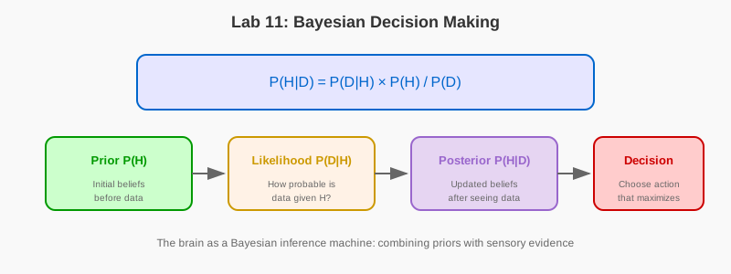
11.1 Learning Objectives
- Implement Bayesian inference for perceptual decisions
- Model prior beliefs and likelihood functions
- Simulate sequential probability ratio test (SPRT)
- Analyze drift-diffusion models of decision making
- Connect Bayesian inference to neural population activity
11.2 Prerequisites
- Reading: Chapter 11: Bayesian Decision Making
- Libraries: NumPy, Matplotlib, SciPy
- Concepts: Bayes’ rule, probability distributions, evidence accumulation
11.3 Setup
import numpy as np
import matplotlib.pyplot as plt
from scipy.stats import norm, beta

np.random.seed(42)
plt.rcParams['figure.figsize'] = (12, 8)
11.4 Part 1: Bayesian Inference
## Simple Bayesian inference example
## Task: Infer orientation from noisy measurements

true_orientation = 45  # degrees
prior_mean = 50
prior_std = 20

## Generate noisy measurements
n_measurements = 5
measurement_noise = 10
measurements = true_orientation + np.random.randn(n_measurements) * measurement_noise

## Bayesian updating
posterior_means = []
posterior_stds = []

prior_precision = 1 / prior_std**2
likelihood_precision = 1 / measurement_noise**2

current_mean = prior_mean
current_precision = prior_precision

for measurement in measurements:
    # Update precision and mean
    current_precision += likelihood_precision
    current_mean = (current_precision - likelihood_precision) / current_precision * current_mean + \
                   likelihood_precision / current_precision * measurement

    posterior_means.append(current_mean)
    posterior_stds.append(1 / np.sqrt(current_precision))

## Visualize
x = np.linspace(0, 100, 1000)
plt.figure(figsize=(14, 8))

## Prior
prior = norm.pdf(x, prior_mean, prior_std)
plt.plot(x, prior, 'b--', linewidth=2, label=f'Prior (μ={prior_mean})', alpha=0.7)

## Plot posteriors after each measurement
colors = plt.cm.RdYlGn(np.linspace(0.3, 0.9, n_measurements))
for i, (mean, std, color) in enumerate(zip(posterior_means, posterior_stds, colors)):
    posterior = norm.pdf(x, mean, std)
    plt.plot(x, posterior, color=color, linewidth=2, label=f'After meas {i+1}', alpha=0.8)

plt.axvline(true_orientation, color='red', linestyle=':', linewidth=2, label='True value')
plt.xlabel('Orientation (degrees)', fontsize=12)
plt.ylabel('Probability Density', fontsize=12)
plt.title('Bayesian Updating with Sequential Measurements', fontweight='bold', fontsize=14)
plt.legend()
plt.grid(True, alpha=0.3)
plt.tight_layout()
plt.show()

print(f"Final estimate: {posterior_means[-1]:.2f} ± {posterior_stds[-1]:.2f}")
print(f"True value: {true_orientation}")
11.5 Part 2: Bayesian Coin Flip Experiment
This exercise demonstrates Bayesian inference for estimating the bias of a coin using conjugate priors (Beta-Binomial).
Run this cell to visualize how posterior beliefs evolve as evidence accumulates.
def bayesian_coin_flip(n_flips=20, true_prob=0.7, show_animation=False):
    """
    Demonstrate Bayesian inference for estimating the bias of a coin.

    Prior: Beta(2, 2) - slightly peaked at 0.5
    Likelihood: Binomial(n_flips, θ)
    Posterior: Beta(α + n_heads, β + n_tails)

    This is conjugate: Beta prior + Binomial likelihood = Beta posterior
    """
    np.random.seed(42)

    # Generate coin flips
    flips = np.random.rand(n_flips) < true_prob  # True if heads
    n_heads = np.cumsum(flips)
    n_tails = np.arange(1, n_flips+1) - n_heads

    # Prior parameters (Beta distribution)
    alpha_prior = 2
    beta_prior = 2

    # Create θ values for plotting
    theta = np.linspace(0, 1, 1000)

    # Plot evolution of belief
    fig, axes = plt.subplots(2, 2, figsize=(14, 10))
    axes = axes.ravel()

    plot_points = [0, 4, 9, n_flips-1]  # Which flips to show

    for idx, flip_idx in enumerate(plot_points):
        ax = axes[idx]

        if flip_idx == 0:
            # Prior only
            alpha_post = alpha_prior
            beta_post = beta_prior
            n_h = 0
            n_t = 0
        else:
            # Posterior after flip_idx flips
            alpha_post = alpha_prior + n_heads[flip_idx]
            beta_post = beta_prior + n_tails[flip_idx]
            n_h = n_heads[flip_idx]
            n_t = n_tails[flip_idx]

        # Plot posterior
        post_dist = beta.pdf(theta, alpha_post, beta_post)
        ax.plot(theta, post_dist, 'b-', linewidth=2, label='Posterior')
        ax.fill_between(theta, post_dist, alpha=0.3, color='blue')

        # True value
        ax.axvline(true_prob, color='red', linestyle='--',
                   linewidth=2, label=f'True θ = {true_prob}')

        # MAP estimate
        map_estimate = (alpha_post - 1) / (alpha_post + beta_post - 2)
        ax.axvline(map_estimate, color='green', linestyle='-',
                   linewidth=2, label=f'MAP = {map_estimate:.2f}')

        ax.set_xlabel('θ (Probability of Heads)')
        ax.set_ylabel('Probability Density')
        ax.set_title(f'After {n_h} heads, {n_t} tails')
        ax.legend()
        ax.grid(alpha=0.3)
        ax.set_ylim(0, ax.get_ylim()[1] * 1.1)

    plt.tight_layout()

    print(f"True probability: {true_prob}")
    print(f"Final MAP estimate: {map_estimate:.3f}")
    print(f"Final posterior: Beta({alpha_post}, {beta_post})")

    return alpha_post, beta_post

# Run the Bayesian coin flip experiment
bayesian_coin_flip(n_flips=20, true_prob=0.7)
Key Insight: As we gather more evidence (flips), the posterior becomes more concentrated around the true value. The prior matters most when data is scarce, but eventually the data overwhelms the prior.
11.6 Part 3: Multisensory Integration
This exercise demonstrates optimal Bayesian cue integration for combining visual and haptic sensory information.
Run this cell to see how the brain optimally weights sensory cues based on their reliability.
def multisensory_integration():
    """
    Demonstrate optimal Bayesian cue integration.

    Scenario: Estimate object size using vision and touch.
    - Visual estimate: noisy but available
    - Haptic (touch) estimate: also noisy
    - Optimal strategy: weight by reliability (inverse variance)
    """
    np.random.seed(42)

    # True object size
    true_size = 10.0  # cm

    # Generate repeated measurements
    n_trials = 100

    # Visual measurements (more variable)
    visual_noise_std = 2.0
    visual_estimates = true_size + np.random.randn(n_trials) * visual_noise_std

    # Haptic measurements (less variable)
    haptic_noise_std = 1.0
    haptic_estimates = true_size + np.random.randn(n_trials) * haptic_noise_std

    # Optimal Bayesian combination
    visual_precision = 1 / visual_noise_std**2
    haptic_precision = 1 / haptic_noise_std**2

    w_visual = visual_precision / (visual_precision + haptic_precision)
    w_haptic = haptic_precision / (visual_precision + haptic_precision)

    combined_estimates = w_visual * visual_estimates + w_haptic * haptic_estimates

    # Sub-optimal: equal weighting
    equal_weight_estimates = 0.5 * visual_estimates + 0.5 * haptic_estimates

    # Visualization
    fig, axes = plt.subplots(1, 2, figsize=(14, 6))

    # Plot 1: Individual and combined estimates
    axes[0].scatter(visual_estimates, haptic_estimates, alpha=0.3, c='gray')
    axes[0].scatter(combined_estimates.mean(), combined_estimates.mean(),
                   s=200, c='green', marker='*', label='Bayesian combined',
                   edgecolors='black', linewidths=2)
    axes[0].scatter(true_size, true_size, s=200, c='red', marker='X',
                   label='True value', edgecolors='black', linewidths=2)
    axes[0].set_xlabel('Visual Estimate (cm)')
    axes[0].set_ylabel('Haptic Estimate (cm)')
    axes[0].set_title('Multisensory Integration')
    axes[0].legend()
    axes[0].grid(alpha=0.3)
    axes[0].axis('equal')

    # Plot 2: Error distributions
    visual_errors = np.abs(visual_estimates - true_size)
    haptic_errors = np.abs(haptic_estimates - true_size)
    combined_errors = np.abs(combined_estimates - true_size)
    equal_errors = np.abs(equal_weight_estimates - true_size)

    positions = [1, 2, 3, 4]
    data = [visual_errors, haptic_errors, combined_errors, equal_errors]
    labels = ['Visual - only', 'Haptic - only', 'Bayesian - combined', 'Equal - weight']

    bp = axes[1].boxplot(data, positions=positions, labels=labels,
                         patch_artist=True, widths=0.6)

    colors = ['#cc0000', '#0066cc', '#00cc00', '#cccccc']
    for patch, color in zip(bp['boxes'], colors):
        patch.set_facecolor(color)
        patch.set_alpha(0.7)

    axes[1].set_ylabel('Absolute Error (cm)')
    axes[1].set_title('Estimation Error by Strategy')
    axes[1].grid(alpha=0.3, axis='y')

    plt.tight_layout()

    print(f"Visual weight: {w_visual:.3f}")
    print(f"Haptic weight: {w_haptic:.3f}")
    print(f" - Mean absolute errors:")
    print(f"  Visual only: {visual_errors.mean():.3f} cm")
    print(f"  Haptic only: {haptic_errors.mean():.3f} cm")
    print(f"  Bayesian combined: {combined_errors.mean():.3f} cm")
    print(f"  Equal weight: {equal_errors.mean():.3f} cm")

    return w_visual, w_haptic

# Run the multisensory integration experiment
multisensory_integration()
Neuroscience Evidence: Ernst & Banks (2002) showed that humans optimally combine visual and haptic cues for size estimation, with weights matching the Bayesian prediction.
11.7 Part 4: Perceptual Decision Making
This exercise simulates Bayesian perceptual decision making with evidence accumulation and confidence thresholds.
Run this cell to visualize how evidence accumulates over time and how posterior beliefs update.
def perceptual_decision_making():
    """
    Simulate Bayesian perceptual decision making.

    Task: Decide whether a noisy stimulus is 'A' or 'B'
    - Collect evidence over time
    - Update posterior probability
    - Make decision when confidence threshold is reached
    """
    np.random.seed(42)

    # True stimulus (0 = A, 1 = B)
    true_stimulus = 1

    # Evidence parameters
    n_timesteps = 50
    if true_stimulus == 0:
        evidence_mean = -0.3  # Evidence favors A
    else:
        evidence_mean = +0.3  # Evidence favors B
    evidence_std = 1.0

    # Prior (equal probability)
    prior_A = 0.5
    prior_B = 0.5

    # Collect evidence over time
    evidence = evidence_mean + np.random.randn(n_timesteps) * evidence_std
    cumulative_evidence = np.cumsum(evidence)

    # Update posterior using Bayesian inference
    # For simplicity, using a diffusion model approximation
    posterior_B = np.zeros(n_timesteps)
    log_posterior_ratio = np.zeros(n_timesteps)

    for t in range(n_timesteps):
        # Log likelihood ratio
        log_lr = cumulative_evidence[t] / evidence_std**2

        # Log posterior ratio (log odds)
        log_posterior_ratio[t] = log_lr + np.log(prior_B / prior_A)

        # Convert to probability
        posterior_B[t] = 1 / (1 + np.exp(-log_posterior_ratio[t]))

    # Decision rule: choose when posterior exceeds threshold
    confidence_threshold = 0.95
    decision_time = np.where(posterior_B > confidence_threshold)[0]

    if len(decision_time) > 0:
        decision_time = decision_time[0]
        decision = 'B'
    elif len(np.where(posterior_B < 1 - confidence_threshold)[0]) > 0:
        decision_time = np.where(posterior_B < 1 - confidence_threshold)[0][0]
        decision = 'A'
    else:
        decision_time = n_timesteps - 1
        decision = 'B' if posterior_B[-1] > 0.5 else 'A'

    # Visualization
    fig, axes = plt.subplots(2, 1, figsize=(12, 10))

    # Plot 1: Evidence accumulation
    axes[0].plot(cumulative_evidence, 'b-', linewidth=2, label='Cumulative evidence')
    axes[0].axhline(0, color='gray', linestyle='--', alpha=0.5)
    axes[0].axvline(decision_time, color='red', linestyle='--',
                    label=f'Decision time = {decision_time}')
    axes[0].set_xlabel('Time (ms)')
    axes[0].set_ylabel('Cumulative Evidence')
    axes[0].set_title('Evidence Accumulation Over Time')
    axes[0].legend()
    axes[0].grid(alpha=0.3)

    # Plot 2: Posterior probability
    axes[1].plot(posterior_B, 'g-', linewidth=2, label='P(stimulus = B | evidence)')
    axes[1].axhline(0.5, color='gray', linestyle='--', alpha=0.5, label='Chance')
    axes[1].axhline(confidence_threshold, color='red', linestyle=':',
                    alpha=0.7, label=f'Threshold = {confidence_threshold}')
    axes[1].axhline(1 - confidence_threshold, color='red', linestyle=':', alpha=0.7)
    axes[1].axvline(decision_time, color='red', linestyle='--')
    axes[1].set_xlabel('Time (ms)')
    axes[1].set_ylabel('Posterior Probability')
    axes[1].set_title('Bayesian Belief Update')
    axes[1].set_ylim(0, 1)
    axes[1].legend()
    axes[1].grid(alpha=0.3)

    plt.tight_layout()

    correct = (decision == 'B' and true_stimulus == 1) or (decision == 'A' and true_stimulus == 0)
    print(f"True stimulus: {'B' if true_stimulus == 1 else 'A'}")
    print(f"Decision: {decision}")
    print(f"Decision time: {decision_time} ms")
    print(f"Correct: {correct}")

    return decision, decision_time

# Run the perceptual decision making simulation
perceptual_decision_making()
Connection to Neuroscience: This model resembles the drift-diffusion model, which accurately describes reaction times and choice behavior in perceptual decision-making tasks. Neural recordings in areas like LIP and FEF show evidence accumulation patterns matching this model.
11.8 Part 5: Probabilistic Population Codes
This exercise demonstrates how neural populations can encode probability distributions.
Run this cell to see how population activity represents posterior beliefs and how to decode them.
def probabilistic_population_code():
    """
    Demonstrate how a neural population can encode a probability distribution.

    Population coding: Each neuron has a preferred stimulus value (tuning curve)
    Population activity pattern represents posterior distribution
    """
    np.random.seed(42)

    # Stimulus space
    stimulus_values = np.linspace(0, 180, 100)  # Orientation in degrees

    # Neural population
    n_neurons = 20
    preferred_orientations = np.linspace(0, 180, n_neurons)
    tuning_width = 20  # degrees

    # True stimulus
    true_orientation = 90

    # Noisy sensory input
    noisy_measurement = true_orientation + np.random.randn() * 10

    # Generate population response
    def tuning_curve(stimulus, preferred, width):
        """Gaussian tuning curve."""
        return np.exp(-0.5 * ((stimulus - preferred) / width)**2)

    population_response = np.zeros(n_neurons)
    for i in range(n_neurons):
        mean_response = tuning_curve(noisy_measurement,
                                     preferred_orientations[i],
                                     tuning_width)
        # Add Poisson noise
        population_response[i] = np.random.poisson(mean_response * 100)

    # Decode: Reconstruct probability distribution from population
    likelihood = np.zeros(len(stimulus_values))
    for i in range(n_neurons):
        # Each neuron votes for stimuli near its preferred orientation
        contribution = tuning_curve(stimulus_values,
                                   preferred_orientations[i],
                                   tuning_width)
        likelihood += contribution * population_response[i]

    # Normalize to get posterior (assuming flat prior)
    posterior = likelihood / likelihood.sum()

    # Maximum a posteriori (MAP) estimate
    map_estimate = stimulus_values[np.argmax(posterior)]

    # Visualization
    fig, axes = plt.subplots(2, 1, figsize=(12, 10))

    # Plot 1: Population response
    axes[0].bar(preferred_orientations, population_response,
               width=8, color='#cc0000', alpha=0.7)
    axes[0].axvline(true_orientation, color='green', linestyle='--',
                   linewidth=2, label=f'True orientation = {true_orientation}°')
    axes[0].set_xlabel('Preferred Orientation (degrees)')
    axes[0].set_ylabel('Spike Count')
    axes[0].set_title('Neural Population Response')
    axes[0].legend()
    axes[0].grid(alpha=0.3, axis='y')

    # Plot 2: Decoded posterior
    axes[1].plot(stimulus_values, posterior, 'b-', linewidth=2,
                label='Decoded posterior')
    axes[1].fill_between(stimulus_values, posterior, alpha=0.3, color='blue')
    axes[1].axvline(true_orientation, color='green', linestyle='--',
                   linewidth=2, label=f'True = {true_orientation}°')
    axes[1].axvline(map_estimate, color='red', linestyle='-',
                   linewidth=2, label=f'MAP = {map_estimate:.1f}°')
    axes[1].set_xlabel('Orientation (degrees)')
    axes[1].set_ylabel('Probability Density')
    axes[1].set_title('Decoded Posterior Distribution')
    axes[1].legend()
    axes[1].grid(alpha=0.3)

    plt.tight_layout()

    print(f"True orientation: {true_orientation}°")
    print(f"Noisy measurement: {noisy_measurement:.1f}°")
    print(f"MAP estimate: {map_estimate:.1f}°")
    print(f"Estimation error: {abs(map_estimate - true_orientation):.1f}°")

    return population_response, posterior

# Run the probabilistic population code simulation
probabilistic_population_code()
11.9 Part 6: Drift-Diffusion Model
def drift_diffusion_trial(drift_rate=0.3, noise=1.0, threshold=1.0, dt=0.01):
    """Simulate single DDM trial."""
    evidence = 0
    time = 0
    evidence_trace = [0]
    time_trace = [0]

    while abs(evidence) < threshold and time < 5:
        evidence += drift_rate * dt + np.sqrt(dt) * noise * np.random.randn()
        time += dt
        evidence_trace.append(evidence)
        time_trace.append(time)

    decision = 1 if evidence > 0 else 0
    return decision, time, evidence_trace, time_trace

## Simulate many trials
n_trials = 100
drift_rates = [0.1, 0.3, 0.5]

fig, axes = plt.subplots(1, 3, figsize=(16, 5))

for ax, drift in zip(axes, drift_rates):
    for trial in range(20):  # Show 20 example traces
        decision, rt, evidence, time_points = drift_diffusion_trial(drift_rate=drift)
        color = 'green' if decision == 1 else 'red'
        ax.plot(time_points, evidence, color=color, alpha=0.3, linewidth=0.8)

    ax.axhline(y=1, color='black', linestyle='--', label='Upper threshold')
    ax.axhline(y=-1, color='black', linestyle='--', label='Lower threshold')
    ax.axhline(y=0, color='gray', linestyle=':', alpha=0.5)
    ax.set_xlabel('Time (s)', fontsize=11)
    ax.set_ylabel('Evidence', fontsize=11)
    ax.set_title(f'Drift Rate = {drift}', fontweight='bold')
    ax.set_ylim(-1.5, 1.5)
    if ax == axes[0]:
        ax.legend()
    ax.grid(True, alpha=0.3)

plt.suptitle('Drift-Diffusion Model: Evidence Accumulation', fontsize=16, fontweight='bold')
plt.tight_layout()
plt.show()
11.10 Part 7: Speed-Accuracy Tradeoff
## Vary threshold and measure speed vs. accuracy
thresholds = np.linspace(0.3, 2.0, 10)
accuracies = []
reaction_times = []

for threshold in thresholds:
    correct = 0
    rts = []

    for trial in range(200):
        # True drift is positive (correct answer = 1)
        decision, rt, _, _ = drift_diffusion_trial(drift_rate=0.4, threshold=threshold)
        if decision == 1:
            correct += 1
        rts.append(rt)

    accuracies.append(correct / 200)
    reaction_times.append(np.median(rts))

plt.figure(figsize=(14, 6))

plt.subplot(1, 2, 1)
plt.plot(thresholds, accuracies, 'o-', linewidth=2, markersize=8, color='blue')
plt.xlabel('Decision Threshold', fontsize=12)
plt.ylabel('Accuracy', fontsize=12)
plt.title('Accuracy vs. Threshold', fontweight='bold')
plt.grid(True, alpha=0.3)

plt.subplot(1, 2, 2)
plt.plot(reaction_times, accuracies, 'o-', linewidth=2, markersize=8, color='red')
plt.xlabel('Reaction Time (s)', fontsize=12)
plt.ylabel('Accuracy', fontsize=12)
plt.title('Speed-Accuracy Tradeoff', fontweight='bold')
plt.grid(True, alpha=0.3)

plt.tight_layout()
plt.show()
11.11 Exercises
- Implement SPRT for sequential hypothesis testing
- Model change-point detection
- Fit DDM to behavioral data
- Connect neural firing rates to evidence accumulation
11.12 Summary
Implemented Bayesian inference, drift-diffusion models, and explored the speed-accuracy tradeoff in decision making.